Showing posts with label Transact SQL T-SQL. Show all posts

GroupBy Clause - SQL Server vs MySQL

A GROUP BY Clause is used to group the data based on specific columns along with summary information. However there are some differences in usage of this clause in SQL Server and MySQL

Let us create this testing table with some sample data

create table testing
(
    sales_id int,
    product_id char(7),
    sales_date datetime,
    sales_amount decimal(12,2)
)


insert into testing(sales_id,product_id,sales_date,sales_amount)
select 1,'PR00001','2001-01-01',1200.00 union all
select 2,'PR00002','2003-01-21',3000.50 union all
select 3,'PR00002','2003-01-21',2500.00 union all
select 4,'PR00001','2002-02-15',1000.00 union all
select 5,'PR00003','2005-12-19',3000.50 union all
select 6,'PR00003','2006-11-01',8000.00 union all
select 7,'PR00004','2007-04-22',350.00 union all
select 8,'PR00004','2007-04-22',590.00 union all
select 9,'PR00004','2007-04-22',590.00 union all
select 10,'PR00001','2008-05-27',4800.50


If you want to get total sales amount for each product, you can write this query both in SQL Server and MySQL

select product_id,sum(sales_amount) as sales_amount from testing
group by product_id


As per ANSI SQL, all columns that are not part of aggregate functions should be included in GROUP BY clause

If you run the following code in SQL Server

select product_id,sum(sales_amount) as sales_amount from testing

You will get an error

Msg 8120, Level 16, State 1, Line 1
Column 'testing.product_id' is invalid in the select list because it is not contained in either an aggregate function or the GROUP BY clause.


However if you run this code in MySQL, you will get the following result

Product_id        sales_amount
-----------        --------------
PR00001        25031.50

Because MySQL does the auto grouping for the columns specified in the SELECT statement, if they are omitted in GROUP BY clause, it just simply displays the first value of columns along with total of summary column. In this case, it displays the first product id and total of all products

The following is also possible in MySQL

select *,sum(sales_amount) as sales_amount from testing

As explained, it will list out all columns of first row along with total of sales_amount. You need to aware of this feature in MySQL while using GROUP BY Clause

SQL Server Inner Join - Concepts and Best practices

In a database such as SQL Server, we create tables which are related to each other through a common column. For example, if we have to store customers’ related information, then the customer’s personal information gets stored in one table and the same customer’s transaction information, gets stored in another table. Both the tables have CustID as a common column.

We can implement RDBMS (Relational Database Management System) concepts through any database, such as SQL Server. So the same entity’s information flows down in different tables. This is part of the Normalization process within RDBMS framework.

However as part of the requirement, we may need to show a report containing customer information from multiple tables, on a matching column condition. Here arises the need of using the technique of Joins in SQL scripting.

Example - Let us create an Employee specific set of 2 tables in a new database.

Execute the following script in your instance of SQL Server.

Use Master
go
Create Database Inner_Join
go
Use Inner_Join
go
CREATE TABLE EMP
       (EMPNO Integer,
        ENAME Varchar(15),
        JOB Varchar(9),
        MGR Integer,
        HIREDATE datetime,
        SAL Integer,
        COMM Integer,
        DEPTNO Integer)
go
INSERT INTO EMP VALUES
        (7369, 'SMITH', 'CLERK', 7902, '12/17/80', 800, NULL, 20)
INSERT INTO EMP VALUES
        (7499, 'ALLEN', 'SALESMAN', 7698, '5/20/81', 1600, 300, 30)
INSERT INTO EMP VALUES
        (7521, 'WARD', 'SALESMAN', 7698, '5/22/81', 1250, 500, 30)
INSERT INTO EMP VALUES
        (7566, 'JONES', 'MANAGER',   7839, '4/2/81', 2975, NULL, 20)
INSERT INTO EMP VALUES
        (7654, 'MARTIN', 'SALESMAN', 7698, '9/28/81', 1250, 1400, 30)
INSERT INTO EMP VALUES
        (7698, 'BLAKE', 'MANAGER',   7839, '5/1/81', 2850, NULL, 30)
INSERT INTO EMP VALUES
        (7782, 'CLARK', 'MANAGER',   7839, '6/9/81', 2450, NULL, 10)
INSERT INTO EMP VALUES
        (7788, 'SCOTT',  'ANALYST',  7566, '12/9/82', 3000, NULL, 20)
INSERT INTO EMP VALUES
        (7839, 'KING',   'PRESIDENT', NULL, '11/17/81', 5000, NULL, 10)
INSERT INTO EMP VALUES
        (7844, 'TURNER', 'SALESMAN', 7698, '9/8/1981',1500,    0, 30)
INSERT INTO EMP VALUES
        (7876, 'ADAMS', 'CLERK', 7788, '1/12/83', 1100, NULL, 20)
INSERT INTO EMP VALUES
        (7900, 'JAMES', 'CLERK', 7698,  '12/3/81', 950, NULL, 30)
INSERT INTO EMP VALUES
        (7902, 'FORD',   'ANALYST', 7566, '12/3/81', 3000, NULL, 20)
INSERT INTO EMP VALUES
        (7934, 'MILLER', 'CLERK',  7782, '1/23/82', 1300, NULL, 10)
go
CREATE TABLE DEPT
       (DEPTNO INTEGER,
        DNAME VARCHAR(14),
        LOC VARCHAR(13) )
go
INSERT INTO DEPT VALUES (10,'ACCOUNTING','NEW YORK')
INSERT INTO DEPT VALUES (20,'RESEARCH','DALLAS')
INSERT INTO DEPT VALUES (30,'SALES','CHICAGO')
INSERT INTO DEPT VALUES (40,'OPERATIONS','BOSTON')
go

Let us see the tables to understand the relationship.

use Inner_Join
go
select * from dept
go
select * from emp
go

dept-no

You can observe that Deptno is the common field in both the tables, Dept & Emp. Department details are in Dept table and Employee table contains a DEPTNO column which represents the Department Number an Employee belongs to. Let us see two records of Emp table to get a clarity. Consider the record of SMITH in Emp table. Smith’s Deptno is 20, which means Smith’s Department Name (DNAME) is RESEARCH. Similarly consider ALLEN’s record. His Deptno is 30, which means Allen’s DNAME is Sales. So for the first two records, we have mapped the common column Deptno!
Now we want to display the ENAME and DNAME for the matching Deptno. This is possible by a technique within SQL scripting that is called as Joins.

There are multiple types of joins, but in this article we are going to focus on Inner Join or also known as Equi-Join.

Editorial Note: Check this artilce to understand Types of JOIN in SQL Server - Inner, Self, Outer and Cross JOIN

So what is Inner Join? Inner join is displaying data from multiple tables on matching values of common field (s), within the associated tables.

Inner Join Syntax

There are two types of syntaxes for Inner join:

1) Non-ANSI
2) ANSI

Let us see the Non-ANSI syntax first:

select ename, dname
from emp, dept
where emp.deptno = dept.deptno

non-ansi-sql

One thing to note is that in the from clause of SQL statement, we have two tables separated by a comma. The mapping of common column is done in the where clause.

How does it work internally? Whenever a JOIN command is given, then each record of the first table is evaluated with each record of the second table. That means a Cartesian product happens and then as per the matching values of where clause, those records are shown. As per the Emp and Dept tables, 14 records of Emp are cross evaluated with 4 records of Dept table. So overall 14 * 4 = 56 evaluations will happen and matching value records are shown.

Now, let us remove the where clause and see what happens.

select ename, dname
from emp, dept

where-clause
rows-affected

Oops!! The Cartesian product result is displayed now! Due to the absence of where clause, each evaluation has been displayed as well. So this output is logically going wrong! Actually we have accidentally landed in another type of join that is Cross Join.

Now, let us have the common field for display purpose. We will include the Deptno column along with Ename and Dname columns in the column list.

select ename, dname, deptno
from emp, dept
where emp.deptno = dept.deptno

It has thrown the following error –

ambiguous-column

The common field’s name is same in both the tables. So a confusion arose in understanding that deptno from which table should be considered. The error would not have come if the common column had different name. In such a case where name is same, it is mandatory to mention the table name and . (dot) separator as prefix .

Let us rectify the above query.

select ename, dname, emp.deptno
from emp, dept
where emp.deptno = dept.deptno

inner-join-result

Ideally table name prefix should be mentioned for each column irrespective of whether it is common or uncommon. Advantage of this approach is that it will give clarity to any other user who is not habitual with the tables & its columns.

So the same query will be written as follows:

select emp.ename, dept.dname, emp.deptno
from emp, dept
where emp.deptno = dept.deptno

But in projects, table names many a times are lengthy. So mentioning a lengthy table name repeatedly the will be cumbersome. To avoid that, introduce a table alias in the from clause. Use that alias in the column list and where clause.

JOIN – Best practice

So now I am coming to the best practice of writing a JOIN statement.

select e.ename, d.dname, e.deptno
from emp e, dept d
where e.deptno = d.deptno

Internally, from clause is getting executed first, then the where clause and finally the select clause as per the above statement. 

INNER JOIN – ANSI Syntax

So far we have seen the NON-ANSI syntax of joining tables. Now let us see the ANSI syntax. As per ANSI Joins, there are two changes:

1. The comma within from clause gets replaced by Join type specification
2. The JOIN condition has to be given using ON clause instead of where clause.

The select statement will look like this:

select e.ename, d.dname, e.deptno
from emp e Inner Join dept d
On e.deptno = d.deptno

Amongst the multiple types of joins, the default type of join is an Inner Join. So Inner is an optional keyword. The query can have only Join as the keyword which will be as follows: 

select e.ename, d.dname, e.deptno
from emp e Join dept d
On e.deptno = d.deptno 

In Non-ANSI style of join, we have observed that if the where clause is skipped, then it shows a Cartesian product output. On the same lines, let us try to omit the On clause in ANSI and let’s see what happens.

select e.ename, d.dname, e.deptno
from emp e Join dept d

It is throwing an error.

incorrect-syntax

It means that On clause is mandatory in ANSI type of join. The advantage of ANSI join is that it is a dedicated inner join and it prevents an accidental Cartesian product.

About one-to-many relationship for Inner join

The inner or equi join will be logically correct if we have one-to-many relationship between the values of common field. In the Emp and Dept tables, there is such relationship, so the output is correct, i.e a matching deptno is once in the dept table and it is multiple times in the emp table.

What if there is a many-to-many relationship within the tables? Right now the deptno column is not having a primary constraint in the Dept table. So we can add one more record of the same deptno 10.

Insert into Dept Values(10, 'Testing', 'CALIFORNIA')
Go

So right now there are 2 records of the same deptno 10 in dept table.

Let us see that –

select * from dept

duplicate-records

Now we will execute the same ANSI join statement again.

select e.ename, d.dname, e.deptno
from emp e Join dept d
On e.deptno = d.deptno 

The output has logically gone wrong!

wrong-output

CLARK, KING and MILLER are displayed in both Accounting & Testing departments.

An Inner join will give correct result only when there is one-to-many relationship. Therefore normally this problem gets eliminated when we have Primary Key and Foreign Key relationship within the common field.

Let us delete this additional record of deptno 10 so that everything goes back to normal.

Delete from Dept
where DName = 'Testing'
go

Important features of Inner Join

1. Common field name may be same or different.
2. The data type and size of common fields should be ideally the same.
3. If the data type is not same, then using type casting functions the data types should be made same in the On clause.
4. There should be one-to-many relationship within the common field values.
I hope through this article, your Inner Join principle now is as sound as a dollar!

SQL Server Query Pagination

This article was authored by Praveen Dabade.

In SQL Server 2012, Microsoft introduced a couple of T-SQL Enhancements. One of them is Query Pagination which we will explore today.

For this demonstration, I am using the Northwind database to demonstrate this new feature. Now in most of the applications, a common requirement is how to fetch the data from the database servers, page wise.

In earlier versions of SQL Server like SQL Server 2005/2008/R2, we can implement Pagination by using different techniques. For example, we implement pagination using ROW_NUMBER() function or CTE - Common Table Expression.

In SQL Server 2012, Microsoft has introduced Pagination as a part of Select query in a Order By clause. Now you will have to use OFFSET and FETCH NEXT with the order by clause.

Let's take a look at a few examples. I am using Northwind database for this demonstration. I have created a Stored Procedure which takes two parameters. First parameter takes the page number and the second parameter ask you to fetch the no. of records for that page. The stored procedure code is as below -

query-pagination

If you execute the above stored procedure

EXEC FetchPagedRecords 2,10

you will get the following results -

image

The OFFSET specifies the number of rows to skip before it starts returning the rows and FETCH NEXT specifies the number of rows to be returned.

Microsoft has introduced an easy way of implementing Data Paging in SQL Server 2012 by adding OFFSET and FETCH NEXT in an Order By clause. I hope you will use it in your applications.

Shrink a Live SQL Server Database and Logs - Caveats and Best Practices

Updated on December 20th, 2017.

If you have deleted a lot of data in the database and truncated some tables, probably you may want to shrink database files to recover the unused space. Basically shrinking will move the data pages at the end of the file into unoccupied space, available in the front of the file.

You can use the DBCC SHRINKDATABASE command. For example, this command

DBCC SHRINKDATABASE (your_database,10) 

will decrease database size and allow for 10 percent free space. 

You can also shrink log file alone using DBCC SHRINKFILE command Take full back up of the database and run the following :

ALTER DATABASE your_database SET RECOVERY SIMPLE; 

DBCC SHRINKFILE (your_database_Log, 10); 

ALTER DATABASE your_database SET RECOVERY FULL; 

It will set the log file size to 10 MB 

Caveats of shrinking database and logs:

1. SHRINK commands should not be done frequently as it will increase the index fragmentation.

2. It is a fully logged operation which will increase the log size and slows down the performance

3. Shrinking is not possible while the current database is being backed up up or restored

4. Shrinking is not possible when columnstore index is enabled

Best practices

1. Use SHRINK only if a lot of operations such as TRUNCATE and DROP has lead to unused space

2. Take full backup before shrinking database files. If you shrink log file, set the Recovery mode into SIMPLE before shrinking and make it FULL after shrinking

3. Never turn ON AUTO SHRINK option

4. Always rebuild indexes after SHRINKING the database files to avoid fragmentation

SQL Server ISNULL() With Multi Column Names

Many a times we come across null values within tables in SQL Server. Null values are the values with no data; that means the data is missing or unknown. In this article, initially we will understand the SQL Server IsNull function, then we will move towards extending the IsNull functionality using Coalesce function.

Let us see the following example.

create table Identification
(empid Integer,
ename varchar(30) NOT NULL,
passport_number char(15) ,
license_number char(15) ,
pan char(15) ,
credit_card_number char(15) ,
account_number char(15) 
)
insert into identification values(1,'John',null,null,'PN-78654','CC-12345','AN-3456')
insert into identification values(2,'Martin','PS-566774',null,null,null,null)
insert into identification values(3,'Smith',null,null,null,null,null)
insert into identification values(4,'Roger',null,null,null,null,'AN-9876')
insert into identification values(5,'King',null,null,null,'CC-8787','AN-9878')
go
select * from identification
go

sql1-identification-table
Image1-Identification-Table

In the above table, every employee has an identity proof which is either a passport number, license number, pan, credit card or account number.

SQL Server ISNULL() Function Example

Syntax:
IsNull(Parameter1, Value if null)

IsNull function returns the first parameter if it’s not null. If the first parameter is null, then it returns the second parameter.

Suppose we want to see if an employee has a passport or not, here the IsNull function can help us.

See the following example of using SQL Server ISNULL in a Select Statement:

select empid, ename, IsNull(Passport_Number, 'Not Found') 
as 'Passport Status' from identification

sql2-isnull-with-single-column
Image2-IsNull-With-Single-Column

Limitation of IsNull() function:

IsNull function can check only if one value is null. It cannot check null for multiple values. That means it is not capable of handling the functionality of checking if the first parameter is null and then move on to check the next parameter for null.

Now assume that for report generation, we want to get the passport number or license number or pan number etc. for reference purpose. If passport number is null, then we need to extract the license number. If license number is null then pan, if pan is null then account number. If all are null then we need to flag a message ‘Invalid’.

The problem is that IsNull function here needs to be used in a nesting manner.

Let us see the ISNULL being used in a select statement in a nested fashion:

select empid, ename, 
IsNull(Passport_Number,IsNull(License_Number, 
IsNull(PAN, IsNull(Credit_Card_Number, IsNull(Account_Number,'Invalid'))))) 
as "Status"
from identification

sql3-isnull-multiple-columns
Image3-IsNull-Multiple-Columns

In the above select statement, we have used IsNull function 5 times to get the desired output.

ISNULL vs Coalesce Function:

There is an alternative way using another SQL Server function known as Coalesce.

Syntax of Coalesce:
COALESCE( parameter1, parameter2, parameter3,……. parameter_n , default_parameter)

Coalesce can take multiple parameters. It returns the first not null parameter. If all the parameters are null, then it will return the default parameter.

In other words, we can say that coalesce behaves as per the following syntax as well:

CASE
   WHEN (parameter1 IS NOT NULL) THEN expression1
   WHEN (parameter2  IS NOT NULL) THEN expression2
   ...
   ELSE expressionN
END

So instead of nesting IsNull function multiple times, we can use a single coalesce function and get the same output as shown here:

select empid, ename, 
Coalesce(Passport_Number,License_Number,PAN,Credit_Card_Number,Account_Number,'Invalid')
as "Using Coalesce" from identification

sql4-coalesce
Image4-Coalesce


Conclusion:

We have seen how the SQL Server IsNull function is suitable for checking one null value and how usage of coalesce function can eliminate the need of using IsNull function redundantly.

SQL Server T-SQL DateDiff Example

How do we find the difference between two dates in SQL Server. Not just the difference in the number of days, but also number of weeks, months.

The answer is by using DateDiff in SQL Server. Datediff is also suitable for getting the time elapsed between the start and end of a process.

Here are some real life examples of how t-sql datediff can be used to get a date difference:

1. Calculating the number of days remaining for a postpaid mobile service before it expires? Here an Automated system can calculate the date difference in sql and send an SMS to a customer informing him/her of the number of days remaining.

2. Particularly suitable in embedded systems to note the time taken for each process while manufacturing a product.

3. In library management automation to keep track of the number of days a book had been issued to a customer.

4. For daily login-logout required in an electronic attendance software system of any company. The tsql datediff function can be used to calculate the exact working hours of every employee.

The signature of this function is as follows:

DATEDIFF( interval, date1, date2 )

where date 1 & date 2 can be the actual date or a part of date like an year.

Note: date1 should be greater than or equal to date2.

Interval here can be any of the following as shown in the following chart:

t-sql-date-diff
image1-t-sql datediff interval

Let us see some examples to make it more clear and interesting.

select datediff (yy, '1984', '1997')  -- 13 years difference

select datediff (dd, '1984', '1986') -- 731 days difference

select datediff (mm, '1984', '1986') -- 24 months difference

select datediff (qq, '1984', '1986') -- 8 quarters difference

select datediff (hour,'2016/05/02 11:00', '2016/05/02 14:45' 
-- 3 hours difference

Database Oriented Example


The DateDiff SQL function can also be used in a where clause.

Let us create a sample database for the same in our SQL Server instance.

Use Master
go
create database DateDiff_Demo
go
Use DateDiff_Demo
go
create table Compaints_Details
(ComplaintID Integer Identity,
 CustId Varchar(7),
 Complaint_Description Varchar(100),
 Engineer_ID Varchar(4),
 Date_of_Complaint date,
 Date_of_Resolve date
 )
 Insert into Compaints_Details 
(CustiD, Complaint_Description, Engineer_ID, 
 Date_of_Complaint,Date_of_Resolve)
 Values
 ('C1', 'Modem problem', 'E1', '21-Apr-2016', '24-Apr-2016')

 Insert into Compaints_Details 
(CustiD, Complaint_Description, Engineer_ID, 
  Date_of_Complaint,Date_of_Resolve)
 Values
 ('C2', 'Wire Connection problem', 'E1', '22-Apr-2016', '22-Apr-2016')

 Insert into Compaints_Details 
 (CustiD, Complaint_Description, Engineer_ID, 
  Date_of_Complaint,Date_of_Resolve)
 Values
 ('C3', 'Socket problem', 'E1', '23-Apr-2016', '28-Apr-2016')

 Insert into Compaints_Details 
 (CustiD, Complaint_Description, Engineer_ID, 
  Date_of_Complaint,Date_of_Resolve)
 Values
 ('C5', 'LAN problem', 'E1', '29-Apr-2016', '29-Apr-2016')
 GO
 select* from Compaints_Details
 go

sql datediff sample data
Image2-SampleData to run a sql datediff query

Let us say we want to see how many days were elapsed for every complaint to get resolved.

Here we will use the Tsql DateDiff function.

SELECT  [ComplaintID]
      ,[CustId]
      ,[Complaint_Description]
      ,[Engineer_ID]
      ,[Date_of_Complaint]
      ,[Date_of_Resolve]
      , DateDiff(dd, [Date_of_Complaint]
      , [Date_of_Resolve]) as [Days taken to resolve]
FROM [DateDiff_Demo].[dbo].[Compaints_Details]

tsql datediff days
Image3-DaysTaken before a complaint was resolved


Conclusion:


And that’s how we can use the SQL Server T-SQL DateDiff function to calculate the day, month, year, and time part differences between two specified dates.

SQL Server: Return Newly Inserted Row

Whenever you insert a new row in a SQL Server table that contains default values, you may want to return the newly inserted row to the user, along with the default value generated. However while doing a plain INSERT statement, all you get is the total number of rows affected.

Here’s an example:

insert-row

Here we are using the NEWID() to generate a unique customer number in each row. However as you can see, the user does not get to see the default ID that got generated for the newly inserted rows. In order to get back the row values that were inserted, use the OUTPUT clause of the INSERT statement as shown here:

INSERT INTO #TT (Name, AreaCode)
OUTPUT INSERTED.ID, INSERTED.Name, INSERTED.AreaCode
SELECT 'Suprotim', 2355 UNION ALL
SELECT 'Anush', 2388
and this time you get to see the newly inserted rows:

sql-server-output-insert

As you can see, we have added the OUTPUT clause right after the INSERT statement. The rows inserted into the table are captured in the virtual table INSERTED and returned back as a result set.

In case you are wondering, yes it is possible to capture the result set in a table or table variable. Assuming there is a Table variable called @TempTbl, just use the following:

INSERT INTO #TT (Name, AreaCode)
OUTPUT INSERTED.ID, INSERTED.Name, INSERTED.AreaCode
INTO @TempTbl
SELECT 'Suprotim', 2355 UNION ALL
SELECT 'Anush', 2388
and now you can do further processing on this data using @TempTbl.

Calculate SQL Azure Database Size

I was looking out for a correct way to programmatically determine the size of a SQL Azure database. After searching many solutions, I finally found one shared by Dimitri Furman of the SQL Server team.

His solution involves using the sys.database_files dmv and the FILEPROPERTY function with the ‘SpaceUsed’ argument.

To those new to sys.database_files, this system catalog view stores information and properties about each file for a database. Since it is a db-level view, it gives information about files in the current database only. Five properties that could be of interest are: logical filename, physical filename, initial size, maximum size and a growth increment.

To determine how much space is used in a file, you can use FILEPROPERTY with SpaceUsed.

Here’s an example: SELECT FILEPROPERTY(‘SomeFile’, ‘SpaceUsed’); I have often used the FILEPROPERTY function in the past while monitoring the progress of a SHRINK operation.

Query for calculating Size of a SQL Azure Database

Here’s how to combine sys.database_files with FILEPROPERTY to programmatically calculate the size of a SQL Azure database.

SELECT 
SUM(CAST(FILEPROPERTY(name, 'SpaceUsed') AS bigint) * 8192.) 
AS DatabaseSizeInBytes,
SUM(CAST(FILEPROPERTY(name, 'SpaceUsed') AS bigint) * 8192.)/1024 /1024
AS DatabaseSizeInMB,
SUM(CAST(FILEPROPERTY(name, 'SpaceUsed') AS bigint) * 8192.)/1024/1024/1024 
AS DatabaseSizeInGB
FROM sys.database_files
WHERE type_desc = 'ROWS';

Let’s understand this query.

FILEPROPERTY() returns an int value for a file name stored within sys.database_files. Since sys.database_files is a db-level view, it gives information about files in the current database only. If a file is not present, null value is returned.

Since SpaceUsed represents "pages" and a page is 8 KB in SQL Server, so multiplying by 8192 gets the total bytes. Then dividing two times by 1024 converts the output to MB, and dividing by three times by 1024 converts the output to GB.

CAST is for casting the value to type bigint

If anybody is wondering about the dot (.) after an 8192, then it is to convert the result implicitly to a decimal value.

Please note that logs are excluded for the purposes of determining database size.

To know about Azure SQL Database resource limits, check https://docs.microsoft.com/en-in/azure/sql-database/sql-database-resource-limits

Remove Non-Alphabet Characters from a String–SQL Server

Suppose you have a string that contains numbers and other special characters and you want to keep only alphabets and remove all the other characters. One way to do this is to use a while loop that parses each character

Here is the code for the same

declare @str varchar(20)
set @str='ab12#89L(h12k'
Select @str as 'Original String'
declare @temp_str varchar(20), @i int
select @temp_str ='',@i=1
while @i<=len(@str)
begin
    set @temp_str=@temp_str+case when substring(@str,@i,1) like '[a-zA-Z]' then substring(@str,@i,1) else '' end
    set @i=@i+1
end
select @temp_str as 'String with Alphabets'


The code inside the While loop takes each character and check if it is in the range a-z or A-Z and appends that character with another variable. Other characters will not get appended. So at the end of while loop, the second variable will have only alphabets.

image

Nested Case Statement in SQL Server

This article is a continuation of SQL Server CASE Statement and CASE WHEN Examples . Today we will learn about Nested Case Statement in SQL Server.

We can nest CASE statements similar to nested ifs that we find in most programming languages.

Let us see an example.

select ename, job, sal, case  -- Outer Case
    when ename like 'A%' then
    case when sal >= 1500 then 'A' -- Nested Case
    end
    when ename like 'J%' then
    case when sal >= 2900 then 'J' -- Nested Case
    end
end as "Name-Grade"            
From Emp

7-nested-case
Image 7-Nested-Case

Limit of nesting a CASE function is up to 10 levels only.

In the following example, the limit of 10 is completely utilized.

Declare @x int
set @x = 1
Select 
case when @x <= 100 then  -- Level 1
 case when @x <= 90 then -- Level 2
    case when @x <= 80 then -- Level 3
        case when @x <= 70 then -- Level 4
            case when @x <= 60 then -- Level 5
                case when @x <= 50 then -- Level 6
                    case when @x <= 40 then -- Level 7
                       case when @x <= 30 then --Level 8
                         case when @x <= 20 then--Level 9
                           case when @x<= 10 then--Level 10
                                100
End End End End End End End End End 
End as "Nested Case" 
--Ending all levels!

8-nested-case-upto-10-levels
Image 8-Nested-Case-Upto-10-Levels

If nesting is exceeding 10 levels, then SQL Server throws an error.
Declare @x int
set @x = 1
Select 
case when @x <= 100 then  -- Level 1
case when @x <= 90 then -- Level 2
case when @x <= 80 then -- Level 3
    case when @x <= 70 then -- Level 4
        case when @x <= 60 then -- Level 5
            case when @x <= 50 then -- Level 6
                case when @x <= 40 then -- Level 7
                   case when @x <= 30 then --Level 8
                     case when @x <= 20 then--Level 9
                       case when @x<= 10 then--Level 10
                          case when @x <= 11 then -- 11
                             100
End End End End End End End End End End 
End as "Nested Case"

Msg 125, Level 15, State 4, Line 14
Case expressions may only be nested to level 10.

SQL Server select into temp table

Many a times we get an output, and then query the output further. In such scenarios instead of writing the entire query repeatedly, and then improvising it or filtering it differently, we can dump the output of the main query into a temporary table i.e. Select into Temp table. Later we can query the temporary table & improvise the outputs as needed.

Let us create the sample tables.

CREATE TABLE EMP
       (EMPNO Integer Primary Key,
        ENAME Varchar(15),
        JOB Varchar(9),
        MGR Integer,
        HIREDATE datetime,
        SAL Integer,
        COMM Integer,
        DEPTNO Integer);

INSERT INTO EMP VALUES
        (7369, 'SMITH',  'CLERK',     7902, '12/17/80',
        800, NULL, 20);
INSERT INTO EMP VALUES
        (7499, 'ALLEN',  'SALESMAN',  7698,
        '5/20/81',1600,  300, 30);
INSERT INTO EMP VALUES
        (7521, 'WARD',   'SALESMAN',  7698,
        '5/22/81', 1250,  500, 30);
INSERT INTO EMP VALUES
        (7566, 'JONES',  'MANAGER',   7839,
        '4/2/81',  2975, NULL, 20);
INSERT INTO EMP VALUES
        (7654, 'MARTIN', 'SALESMAN',  7698,
        '9/28/81', 1250, 1400, 30);
INSERT INTO EMP VALUES
        (7698, 'BLAKE',  'MANAGER',   7839,
        '5/1/81',  2850, NULL, 30);
INSERT INTO EMP VALUES
        (7782, 'CLARK',  'MANAGER',   7839,
        '6/9/81',  2450, NULL, 10);
INSERT INTO EMP VALUES
        (7788, 'SCOTT',  'ANALYST',   7566,
        '12/9/82', 3000, NULL, 20);
INSERT INTO EMP VALUES
        (7839, 'KING',   'PRESIDENT', NULL,
        '11/17/81', 5000, NULL, 10);
INSERT INTO EMP VALUES
        (7844, 'TURNER', 'SALESMAN',  7698,
        '9/8/1981',  1500,    0, 30);
INSERT INTO EMP VALUES
        (7876, 'ADAMS',  'CLERK',     7788,
        '1/12/83', 1100, NULL, 20);
INSERT INTO EMP VALUES
        (7900, 'JAMES',  'CLERK',     7698,
        '12/3/81',   950, NULL, 30);
INSERT INTO EMP VALUES
        (7902, 'FORD',   'ANALYST',   7566,
        '12/3/81',  3000, NULL, 20);
INSERT INTO EMP VALUES
        (7934, 'MILLER', 'CLERK',     7782,
        '1/23/82', 1300, NULL, 10);


CREATE TABLE DEPT
       (DEPTNO INTEGER Primary Key,
        DNAME VARCHAR(14),
        LOC VARCHAR(13) );

INSERT INTO DEPT VALUES
        (10,'ACCOUNTING','NEW YORK');
INSERT INTO DEPT VALUES (20,'RESEARCH','DALLAS');
INSERT INTO DEPT VALUES
        (30,'SALES','CHICAGO');
INSERT INTO DEPT VALUES
        (40,'OPERATIONS','BOSTON');

Now we will write a complex looking select statement as shown here –

select ename, emp.deptno, sal, 
           case when sal >= 5000 then 'Grade A'
                when sal >= 3000 then 'Grade B'
                when sal >= 2500 then 'Grade C'
                when sal >= 2000 then 'Grade D'
                when sal >= 1000 then 'Grade E'
                else
                'Grade F'
            end as Sal_Grade,
            datepart(yy, hiredate) as Year_Of_Hiredate,
            DName,
           Sal + IsNull(Comm,0) as Total,
           Case
            when Comm is null or Comm = 0 then 'Commission not provided'
            when Comm is not null then 'Commission provided'
            End as Commission_Status,
               SubString(Loc,1,1) as Location_ID
from emp join dept
on Emp.deptno = Dept.deptno

The output of this query is as as follows –

complex-select-output

In this query, we have used the following techniques:

1. Two Case Functions
2. Date Function
3. IsNull Function
4. Substring Function
5. Inner Join

Now improvise this output. Put this output into a local temporary table by issuing the following query:

Select * into #Emp_Info
from(select ename, emp.deptno, sal, 
           case when sal >= 5000 then 'Grade A'
                when sal >= 3000 then 'Grade B'
                when sal >= 2500 then 'Grade C'
                when sal >= 2000 then 'Grade D'
                when sal >= 1000 then 'Grade E'
                else
                'Grade F'
            end as Sal_Grade,
            datepart(yy, hiredate) as Year_Of_Hiredate,
            DName,
           Sal + IsNull(Comm,0) as Total,
           Case
            when Comm is null or Comm = 0 then 'Commision not provided'
            when Comm is not null then 'Commision provided'
            End as Commission_Status,
               SubString(Loc,1,1) as Location_ID
from emp join dept
on Emp.deptno = Dept.deptno
) as Emp_Dept

So now these 14 processed rows are the actual records of #Emp_Info table. Therefore now when we will query this table, the inner join, case, date, substring & IsNull functions do not get executed again & again. This will be a big performance boost!

Let’s explore different outputs querying the #Emp_Info table now.

Query 1 – Display records of Grade B employees

Select * from #Emp_Info
where Sal_Grade = 'Grade B'
go

gradeb-employees
Query 2 – Display grade wise total of salaries

Select Sal_Grade, Sum(Sal) as Salary_Sum
from #Emp_Info
Group by Sal_Grade
go

sql-select-into-temp

Query 3 – Display employee names, totals, DName and year of hiredate for all employees who have joined in 1981.

Select Ename, DName, Total, Year_of_Hiredate
from #Emp_Info
where Year_of_Hiredate = '1981'
sql-select

So as we can see, doing a T-SQL Select into temp table can help us fire additional queries on the output, and in some cases, give a performance boost too

SQL Server Default Port

In this article, we are going to explore the default port number of SQL Server required for getting connected to different applications.

What is a Port? It is an endpoint of communication in an operating system. A port is always associated with an IP address of a host, and the protocol type of the communication, thereby completing the destination or origination address of a communication session. A port is identified for each address and protocol by a 16-bit number, commonly known as the port number.
When front end applications want to connect to SQL Server, port number is essential.

The default port number of SQL Server is 1433.

How to get the port number in SQL Server?

Note - The steps are shown through SQL Server 2012 environment. They are largely applicable to SQL Server 2014 too.

Step 1: Open the SQL Server Configuration Manager window through Start > All Programs > Microsoft SQL Server 2012 > Configuration Tools 

sccm-navigation

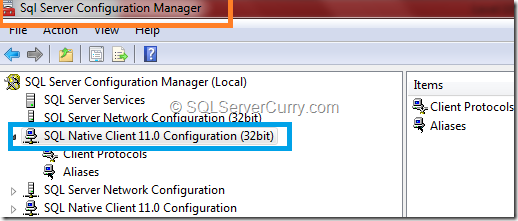
Step 2: Explore SQL Native Client 11.0 Configuration (32bit)

sql-native-client-configuration

Step 3: Click on Client Protocols option within it  –

client-protocols

Step 4: Double click on TCP/IP from the right hand side pane

tcp-ip

We will get to know the Default Port as shown here

1433-default-port

The default port > 1433 port is the official Internet Assigned Number Authority (IANA) socket number for SQL Server. Client systems use TCP 1433 to connect to the database engine; SQL Server Management Studio (SSMS) uses the port to manage SQL Server instances across the network. You can reconfigure SQL Server to listen on a different port, but 1433 is by far the most common implementation.

Some other default SQL Server ports:

TCP 1434 – For Dedicated Admin Connection
UDP 1434 – For SQL Server Named Instance
TCP 2383 – For Default port of SSAS
TCP 2382 – For Named instances of SSAS
TCP 135 – For SSIS & T-SQL Debugger
TCP 80 and 443 – For SSRS
TCP 4022 – For Service Broker

other-default-ports

SQL Server Update statement with JOIN

In this article, we are specifically going to see a practical usage of the UPDATE statement in SQL Server when the condition is based on JOIN of another table.

Example:

CREATE TABLE EMP
       (EMPNO Integer Primary Key,
        ENAME Varchar(15),
        JOB Varchar(9),
        MGR Integer,
        HIREDATE datetime,
        SAL Integer,
        COMM Integer,
        DEPTNO Integer);
go
INSERT INTO EMP VALUES
        (7369, 'SMITH',  'CLERK',     7902, '12/17/80',
        800, NULL, 20);
INSERT INTO EMP VALUES
        (7499, 'ALLEN',  'SALESMAN',  7698,
        '5/20/81',1600,  300, 30);
INSERT INTO EMP VALUES
        (7521, 'WARD',   'SALESMAN',  7698,
        '5/22/81', 1250,  500, 30);
INSERT INTO EMP VALUES
        (7566, 'JONES',  'MANAGER',   7839,
        '4/2/81',  2975, NULL, 20);
INSERT INTO EMP VALUES
        (7654, 'MARTIN', 'SALESMAN',  7698,
        '9/28/81', 1250, 1400, 30);
INSERT INTO EMP VALUES
        (7698, 'BLAKE',  'MANAGER',   7839,
        '5/1/81',  2850, NULL, 30);
INSERT INTO EMP VALUES
        (7782, 'CLARK',  'MANAGER',   7839,
        '6/9/81',  2450, NULL, 10);
INSERT INTO EMP VALUES
        (7788, 'SCOTT',  'ANALYST',   7566,
        '12/9/82', 3000, NULL, 20);
INSERT INTO EMP VALUES
        (7839, 'KING',   'PRESIDENT', NULL,
        '11/17/81', 5000, NULL, 10);
INSERT INTO EMP VALUES
        (7844, 'TURNER', 'SALESMAN',  7698,
        '9/8/1981',  1500,    0, 30);
INSERT INTO EMP VALUES
        (7876, 'ADAMS',  'CLERK',     7788,
        '1/12/83', 1100, NULL, 20);
INSERT INTO EMP VALUES
        (7900, 'JAMES',  'CLERK',     7698,
        '12/3/81',   950, NULL, 30);
INSERT INTO EMP VALUES
        (7902, 'FORD',   'ANALYST',   7566,
        '12/3/81',  3000, NULL, 20);
INSERT INTO EMP VALUES
        (7934, 'MILLER', 'CLERK',     7782,
        '1/23/82', 1300, NULL, 10);
go

CREATE TABLE DEPT
       (DEPTNO INTEGER Primary Key,
        DNAME VARCHAR(14),
        LOC VARCHAR(13) );
go
INSERT INTO DEPT VALUES
        (10,'ACCOUNTING','NEW YORK');
INSERT INTO DEPT VALUES (20,'RESEARCH','DALLAS');
INSERT INTO DEPT VALUES
        (30,'SALES','CHICAGO');
INSERT INTO DEPT VALUES
        (40,'OPERATIONS','BOSTON');

Let us see the two tables.

select * from emp
go
select * from dept
go

emp-dept-table

Here we can see that this is a typical parent-child table relationship. Many a times, the end user wants to see the Employee Names (Enames) and Department Names (Dnames). But for that, they need to surrender to the inner join technique. Right now, only 14 rows are in emp table and 4 rows in dept.

But in a real time production environment, the number of records will be much higher. So this may result into a performance overhead. Therefore the DBA in such scenarios may decide to add the DName column in Emp table itself to eliminate the a JOIN overhead.

Note: Here we are moving towards an intentional De-Normalization technique.

The following ALTER Table command is used for that.

Alter Table Emp
Add Dname Varchar(40)

But now the problem is that for existing records if we see the DName colum, then it will be Null. Let us check it.

select * from emp

sql-adding-dname-column

So now we want to update each Dname as per the Dname of Dept table. For this we will issue the Update statement with join.

Update Emp 
set Dname  = Dept.DName
From Emp, Dept
where Emp.Deptno = Dept.Deptno

Technique: Here the update technique with join is used in the following sequential steps.

1. Every record of Emp is taken.
2. Its deptno is matched with deptno of Dept table.
3. The corresponding DName of Dept table is assigned to that row.
4. Next row of Emp is taken.
5. Step numbers 2 & 3 are repeated.
6. This process continues till the last row is reached by Emp table.

So now let us see the Emp table again.

select * from emp

after-update-with-sql-join

and that’s how we can use the Update statement with JOIN in SQL Server.

SQL Server Substring with CharIndex

In this article we are going to explore the T-SQL function CharIndex and also how to use it with another T-SQL function Substring().

CharIndex: This function returns the location of a substring in a string. By default, it is not case sensitive and is useful to check the position of a particular character or digit in the string. I have seen this function being used in product codes, different types of IDs for validation purpose, or to get some business understanding of that code/ID. Here’s the syntax:

CHARINDEX( Substring or Character, string, [start_position] )

where..

Substring or Character - The string that you want to find. It has to be within string data type family such as char or varchar only.
String - The string or number or an alphanumeric value to search within.
start_position - Optional. The position in string where the search will start. The first position is 1.

The function returns bigint if the expressionToSearch is of varchar(max), nvarchar(max), or varbinary(max) data types; otherwise, it retuns an int.

Substring with CharIndex examples:

select charindex('C','ABCDEF',1) 
-- Returns 3

select charindex('C','ABCDEF') 
-- Still returns 3 as start_position is option, default is 1

select charindex('c','ABCDEF',1) 
-- By default not case sensitive, so returns 3

select charindex('c','ABCDEF' COLLATE Latin1_General_CS_AS) 
–- Returns 0 as lowercase c is not found.

select charindex('Z','ABCDEF',1) 
-- Returns 0 as there is no Z character

select charindex('A','ABCDAEFG',2) 
-- Returns the second position of A, i.e. 5

select charindex('A','ABCDAEFG',9) 
-- Returns 0 as there is no ninth position there is no A

select charindex('4',123456) 
-- Searching from pure numbers, returns 4 as 4 is on fourth position

select charindex('curry','sqlservercurry.com') 
-- It considers the first character of string curry, 
-- i.e. c and then checks the first occurrence, so returns 10

Using CharIndex with Substring:

First let us check the functionality of the Substring function. It extracts a part of the string from the specified position.

Syntax:

Substring(String, Position or Index, Number of characters to extract)
select substring('abcdef', 2, 3) 
-- Returns bcd as 2 is from which position and 3 is number of characters to extract

Now the best usage of CharIndex with Substring is to create a functionality of “Text to Columns”.

That means many a times the names are in the format of “FirstName whitespace LastName” in the same column itself. In such cases, the need is to separate First Name in one column, and Last Name in another column for display purposes.

Consider the following example.

create table Authors
(AuthorID Varchar(2),
 AuthorName Varchar(60)
 )
 go
Insert into Authors Values('A1','Suprotim Agarwal')
Insert into Authors Values('A2','Mahesh Sabnis')
Insert into Authors Values('A3','Mandar Mulay')
go
select * from Authors
go

sql-default-author-table

Now let us say we want to display first name and last name in different columns. For that, we will use the substring function and within it, we will use CharIndex function to know the position number of white space.

See the following query:

select substring(AuthorName,1, charindex(' ',AuthorName)) as [First Name],
substring(AuthorName,(charindex(' ',AuthorName)) + 1, len(AuthorName)) as [Last Name]
from Authors
go

substring-with-charindex

Explanation:

First Name - substring(AuthorName,1, charindex(' ',AuthorName)) means from the first position till the first white space comes extract all the characters.

Last Name - substring(AuthorName,(charindex(' ',AuthorName)) + 1, len(AuthorName)) means to extract from the first white space + 1. Then to extract all remaining characters the len function is used.

And that’s how we use the SQL Server T-SQL Substring function, as well as Substring with CharIndex.

SQL Server Delete Duplicate Rows

There can be two types of duplication of rows in a table

1. Entire row getting duplicated because there is no primary key or unique key.
2. Only primary key or unique key value is different, but remaining all values are same.

Scenario 1: Delete duplicate rows without primary key or unique key.

Let us create the following example.

create table customers1
(CustId Int,
 CustName Varchar(20),
 CustCity Varchar(20),
 Passport_Number Varchar(20))
 go
Insert into customers1 Values(1, 'John', 'Paris', 'P123X78')
Insert into customers1 Values(2, 'Martin', 'London', 'L873X92')
Insert into customers1 Values(3, 'Smith', 'New York', 'N293Y99')
Insert into customers1 Values(1, 'John', 'Paris', 'P123X78')
go
select * from customers1
go

sql-row-duplicate

We want remove one of the duplicate records of John.

By issuing the following summary query, we can see which see which records are duplicate.

select * from customers1
Group by Custid,CustName, CustCity, Passport_Number
Having count(*) > 1

duplicate-row

Now we will add this row to a local temporary table.

Select * into #Temp_customers1 from customers1 where 1 = 2
Insert into #Temp_customers1
select * from customers1
Group by Custid,CustName, CustCity, Passport_Number
Having count(*) > 1

Now the situation is that the duplicate row is in the local temporary table. All we need to now is to delete records from main table customers1 as per matching custid of the local temporary table.

Delete from customers1
where custid in (select Custid from #Temp_customers1)

Will the above query work? Not entirely, as by using the above query, we lost all the duplicate records!! Let us see the table again.

select * from customers1
go

deleting-all-duplicate-rows

Now to keep one record of John, we will take help of the local temporary table again. Let us add the same record from temporary table into customers1 table.

Insert into Customers1
select * from #Temp_customers1
go

Finally we got a single record of John at the end. Let us confirm by seeing the Customers1 table.

select * from customers1
go

removing-duplicate-row

Once done, we can drop the local temporary table.

Scenario 2: Delete duplicate rows where primary key or unique key value is different but remaining values are same.

Let us create the following example.

create table customers2
(CustId Int Primary Key,
 CustName Varchar(20),
 CustCity Varchar(20),
 Passport_Number Varchar(20))
 go
Insert into customers2 Values(1, 'John', 'Paris', 'P123X78')
Insert into customers2 Values(2, 'Martin', 'London', 'L873X92')
Insert into customers2 Values(3, 'Smith', 'New York', 'N293Y99')
Insert into customers2 Values(4, 'John', 'Paris', 'P123X78')
Insert into customers2 Values(5, 'John', 'Paris', 'P123X78')
select * from customers2
go

Here is the same customer’s record, but this time John’s record has been added thrice with different customer ids but same Passport number!

duplicate-rows-different-custids

Scenario 2.a: Delete Duplicate rows but keep one using CTE

We need to use the technique of Self Join initially to check for duplicate records containing different custid but same passport number.

select distinct a.*
from customers2 a join customers2 b
on a.custid <> b.custid and a.CustName =  b.CustName
and a.CustCity = b.CustCity  and a.Passport_Number =  b.Passport_Number

selfjoin-showing-duplicate-rows


Now we have realized that custid 1, 4 & 5 are duplicate. The self-join statement accompanied by delete statement will give us the desired output of keeping the last duplicate record by eliminating all the previous duplicate records. We will use the Common Table Expression (CTE) and put the Self Join query in it.

With Duplicates as
(select distinct a.custid as Customer_ID
from customers2 a join customers2 b
on a.custid <> b.custid and a.CustName =  b.CustName
and a.CustCity = b.CustCity  and a.Passport_Number =  b.Passport_Number
) 
Delete from Customers2
where custid in (select Customer_ID from Duplicates)
and custid <> (select max(Customer_ID) from Duplicates)
Let’s check which rows got deleted.
select * from customers2
go

keeping-last-record

Scenario 2.b: Delete all duplicate records but keep the first original one

Let’s first truncate the customers2 table and add the same rows again.

Truncate Table customers2
go
Insert into customers2 Values(1, 'John', 'Paris', 'P123X78')
Insert into customers2 Values(2, 'Martin', 'London', 'L873X92')
Insert into customers2 Values(3, 'Smith', 'New York', 'N293Y99')
Insert into customers2 Values(4, 'John', 'Paris', 'P123X78')
Insert into customers2 Values(5, 'John', 'Paris', 'P123X78')
go

The only change in the sub query will be that we need to use min(CustomerID) instead of max(CustomerID).

So the query will be as follows.

With Duplicates as
(select distinct a.custid as Customer_ID
from customers2 a join customers2 b
on a.custid <> b.custid and a.CustName =  b.CustName
and a.CustCity = b.CustCity  and a.Passport_Number =  b.Passport_Number
) 
Delete from Customers2
where custid in (select Customer_ID from Duplicates)
and custid <> (select min(Customer_ID) from Duplicates)
Let us confirm this in the customers2 table.
select * from customers2
go

keeping-first-record


And that’s how we can delete duplicate records in SQL Server with tables without primary key, containing primary key and by keeping one original row.

T-SQL Insert Into Table Examples

In T-SQL, to add records into a table (SQL Server) we use a Data Manipulation Language (DML) command known as Insert statement. In this article, we are going to explore the different capabilities of the T-SQL Insert statement.

Let us create a table Table1 with 3 columns A, B and C

create table Table1
(A int,
 B Varchar(10),
 C Date)

Example 1: Add one complete row, date in American format

Here we will mention the actual column values in the Values clause in a sequence that matches the columns mentioned in the CREATE TABLE statement.

Syntax: Insert into Table_Name Values(Col1 Value, Col2 Value….., Coln Value)

Insert into Table1 Values (1,'Aa', '12/13/2014')

Example 2: Add one complete row, date in British format

The date can be entered either in American or British format.

Insert into Table1 Values (2,'Bb', '13-Dec-2014')

Example 3: Add one partial row, specifying Null
Sometimes we do not want to add values in every column. Let us create a new row by specifying values for A and C columns only.

Insert into Table1 Values (3, Null, '14-Dec-2014') 

Example 4: Add one partial row, specifying column names

Consider there are 25 columns in a SQL table, and we want to create a new row by specifying values for only 3 columns. In that case, mentioning Null for the remaining 22 columns multiple times will be cumbersome. So instead of that, we can only mention those 3 columns after the table name, and mention the values for only those 3 columns. The remaining 22 columns by default will get null values. Caution: There should not be primary key or NOT NULL constraint to any of those columns.

Syntax: Insert into Table_Name (Column1, Column3, Column5) Values(Col1 Value, Col3 Value, Col5 Value)

Insert into Table1(A,C) Values (4,'15-Dec-2014')

Note: The columns can be mentioned in any sequence after the table name, but then the values need to mentioned in the same sequence.

Example 5: Ignore the identity column while adding row.

If the table has identity (auto number generation property) column, then by default we cannot add value to that column.

Let us create table Table2 with A as identity column and B, C as integer data type columns

create table Table2
(A int identity,
 B int,
 C int)

To add a record, use the syntax demoed in Example 4.

Insert into Table2 (B,C) Values(100,200)

Example 6: Ignore the computed column while adding row

Let us create table Table3 with a,b and c as 3 columns. C will be the computed column.

create table Table3
(A int,
 B int,
 C as (a + b))
Insert into Table3 Values(200, 300)

The column C will implicitly get value 500!

Example 7: Bulk Insertion – Select along with Union All

If we want to add many records in a table through one statement, then SELECT statement can be associated with INSERT statement instead of values clause.

Let us create table Table4 first.

create table Table4
(a int, b varchar(10)
)

Now if we want add five rows in Table4, we will use SELECT statement along with UNION ALL.

Insert into Table4
Select 1,'A'
Union All
Select 2,'B'
Union All
Select 3,'C'
Union All
Select 4,'D'
Union All
Select 5,'E'

Example 8: Bulk Insertion – Select along with Union All, violation of constraint

If any record violates the constraint, then the entire set gets rejected.

create table Table5
(a int check (a <= 3), b varchar(10)
)
Insert into Table5
Select 1,'A'
Union All
Select 2,'B'
Union All
Select 3,'C'
Union All
Select 4,'D'
Union All
Select 5,'E'

No rows will get added in Table 5.

Example 9: Bulk Insertion – Multiple rows through Values clause itself

From SQL Server 2008 version onwards, the Values clause has been strengthen to add multiple rows.

Syntax:

Insert Into TableName
Values    (……………..),
           (……………..),
           (……………..),
           (……………..)

So in the Table4 now, we will add three records using the Values clause.

Insert into Table4
Values (6,'E'),(7,'F'),(8,'G')

Note: If any one record fails then the entire batch gets rejected.

Example 10: Bulk Insertion – Copying records of another table

Many a times we need to copy records from one table to another.

Insert into Target_Table
Select * from Source_Table

Note: Here it is assumed that the structure of source & target tables are same. That means the number of columns should be same, and positional columns should be compatible as per data type & size.
Let us create table Table6 similar to Table4

create table Table6
(a int, b varchar(10)
)

Now all records of Table4 need to be inserted in Table6.

Insert into Table6
Select * from Table4


Example 11: Bulk Insertion – Copying records of another table, but not in all columns.

Let us create table Table7 similar to Table4

create table Table7
(a int, b varchar(10)
)

Here we need to mention the column names. Suppose we want to add records, but taking values of column B only, then the command will be:

Insert into Table7(B)
Select B from Table4

Conclusion:


In this article we have seen how to add records into an SQL Server table using the T-SQL Insert statement with its multiple examples.

SQL Server Alter Table with Add Column

There are many scenarios where we need to do structural changes to a table, i.e. adding a column, modifying data type, dropping a column and so on. This change to an existing table is possible by issuing a SQL Server Data Definition Language (DDL) T-SQL command known as Alter Table.

In this article we are specifically focusing on adding a new column in a table using SQL Server Alter Table.

Scenario 1: Adding columns to empty table

When the table is created and if there are no records in that table, then there is no problem in adding a column or multiple columns to that table.

Let us see the following example:

create table customers1
(
  custid varchar(5),
 custname varchar(50)
)
go

Scenario 1.a: Adding single column:

After creating the table, we realize that date of birth (DOB) column needs to be added. The following command will help us in achieving this.

Alter Table customers1
Add DOB Date
go

Scenario 1.b: Adding multiple columns:

Adding two more columns is also very easy. Let us add nationality and gender as two more columns by just having a comma separator in each definition.

Alter Table customers1
Add Nationality Varchar(40), Gender Char(1)
go

Scenario 1.c: Adding columns with constraints:

Adding a column with constraint such as primary key, unique key, foreign key, not null, check or default is again not challenging in an empty table.

Note – A primary key constraint cannot be added on the new column if there is already a primary key on any other existing column.

Let us add SSN and deposit amount as two columns, SSN having primary key and deposit amount having check constraint.

Alter Table customers1
Add SSN Varchar(10) Primary Key, 
Deposit_Amount Integer Check(Deposit_Amount >= 200)
go

Scenario 2: Adding columns to table having records

When a column is added to a table with existing records, then for those records, by default a null value is assigned by SQL Server.

Adding column on table having existing records.

Let us create table customers2 and add 2 records in it.

create table customers2
(custid varchar(5),
 custname varchar(50)
 )
 Go
Insert into customers2 Values('C1','John')
Insert into customers2 Values('C2','Martin')
go

Scenario 2.a: Adding columns with default null values on existing records.

Alter Table customers2
Add DOB Date
go

Let us see the table Customers2

select * from customers2

sqlserver-nulls-new-column
Image2-No-Default-Value

Scenario 2.b: Adding columns with default value

It might happen that you want to add a column specifying some default value and there are existing records in the table. But in the default setup, those existing records will not get that value.
Let us add token amount as a column to this Customers2 table with default value as 100.

Alter Table customers2
Add Token_Amount Integer Default 100
go

Let us see the table Customers2

select * from customers2

sql-no-default-value
Image2-No-Default-Value

Note -The default value will be effective when new record is added.

Scenario 2.c: Adding columns with default value and applying those values on existing records.

Let us add another column tax with default value as 50. This value needs to be added to the existing records as well. We need to explicitly specify the clause With Values.


Alter Table customers2
Add Tax Integer Default 50 With Values
go

default-value-withclause
Image3-Default-Value-WithClause

Scenario 2.d: Adding columns with Not Null constraint on existing records.

Let us add a column Country with Not Null constraint. Now this will be contradictory because the earlier two records cannot have null value for Country.

Let us try.

Alter Table customers2
Add Country Varchar(50) Not Null
go

It will throw the following error.

ALTER TABLE only allows columns to be added that can contain nulls

To rectify this, we need to mention the default value which will safeguard the earlier records.

Scenario 2.e: Adding columns with not null constraint and default value on existing records

Let’s have India as the default value.

Alter Table customers2
Add Country Varchar(50) Default 'India' Not Null
go

Now this works fine. Let us see the table again.

select * from customers2

default-value-notnull
Image4-Default-Value-NotNull


Conclusion:

In this article, we have seen the following scenarios of using ALTER table to add column to a SQL Server table:

1. Adding one or multiple columns to an empty table.
2. Adding column to table having records. Those records get default value as null.
3. Adding column with default value to table having records
  • In absence of With Values clause
  • In presence of With Values clause
4. Adding column with not null constraint to table having records
  • In absence of Default clause
  • In presence of Default clause