SQL Server Inner Join - Concepts and Best practices

In a database such as SQL Server, we create tables which are related to each other through a common column. For example, if we have to store customers’ related information, then the customer’s personal information gets stored in one table and the same customer’s transaction information, gets stored in another table. Both the tables have CustID as a common column.

We can implement RDBMS (Relational Database Management System) concepts through any database, such as SQL Server. So the same entity’s information flows down in different tables. This is part of the Normalization process within RDBMS framework.

However as part of the requirement, we may need to show a report containing customer information from multiple tables, on a matching column condition. Here arises the need of using the technique of Joins in SQL scripting.

Example - Let us create an Employee specific set of 2 tables in a new database.

Execute the following script in your instance of SQL Server.

Use Master
go
Create Database Inner_Join
go
Use Inner_Join
go
CREATE TABLE EMP
       (EMPNO Integer,
        ENAME Varchar(15),
        JOB Varchar(9),
        MGR Integer,
        HIREDATE datetime,
        SAL Integer,
        COMM Integer,
        DEPTNO Integer)
go

INSERT INTO EMP VALUES
        (7369, 'SMITH', 'CLERK', 7902, '12/17/80', 800, NULL, 20)
INSERT INTO EMP VALUES
        (7499, 'ALLEN', 'SALESMAN', 7698, '5/20/81', 1600, 300, 30)
INSERT INTO EMP VALUES
        (7521, 'WARD', 'SALESMAN', 7698, '5/22/81', 1250, 500, 30)
INSERT INTO EMP VALUES
        (7566, 'JONES', 'MANAGER',   7839, '4/2/81', 2975, NULL, 20)
INSERT INTO EMP VALUES
        (7654, 'MARTIN', 'SALESMAN', 7698, '9/28/81', 1250, 1400, 30)
INSERT INTO EMP VALUES
        (7698, 'BLAKE', 'MANAGER',   7839, '5/1/81', 2850, NULL, 30)
INSERT INTO EMP VALUES
        (7782, 'CLARK', 'MANAGER',   7839, '6/9/81', 2450, NULL, 10)
INSERT INTO EMP VALUES
        (7788, 'SCOTT',  'ANALYST',  7566, '12/9/82', 3000, NULL, 20)
INSERT INTO EMP VALUES
        (7839, 'KING',   'PRESIDENT', NULL, '11/17/81', 5000, NULL, 10)
INSERT INTO EMP VALUES
        (7844, 'TURNER', 'SALESMAN', 7698, '9/8/1981',1500,    0, 30)
INSERT INTO EMP VALUES
        (7876, 'ADAMS', 'CLERK', 7788, '1/12/83', 1100, NULL, 20)
INSERT INTO EMP VALUES
        (7900, 'JAMES', 'CLERK', 7698,  '12/3/81', 950, NULL, 30)
INSERT INTO EMP VALUES
        (7902, 'FORD',   'ANALYST', 7566, '12/3/81', 3000, NULL, 20)
INSERT INTO EMP VALUES
        (7934, 'MILLER', 'CLERK',  7782, '1/23/82', 1300, NULL, 10)

go
CREATE TABLE DEPT
       (DEPTNO INTEGER,
        DNAME VARCHAR(14),
        LOC VARCHAR(13) )
go
INSERT INTO DEPT VALUES (10,'ACCOUNTING','NEW YORK')
INSERT INTO DEPT VALUES (20,'RESEARCH','DALLAS')
INSERT INTO DEPT VALUES (30,'SALES','CHICAGO')
INSERT INTO DEPT VALUES (40,'OPERATIONS','BOSTON')
go

Let us see the tables to understand the relationship.

use Inner_Join
go
select * from dept
go
select * from emp
go

You can observe that Deptno is the common field in both the tables, Dept & Emp. Department details are in Dept table and Employee table contains a DEPTNO column which represents the Department Number an Employee belongs to. Let us see two records of Emp table to get a clarity. Consider the record of SMITH in Emp table. Smith’s Deptno is 20, which means Smith’s Department Name (DNAME) is RESEARCH. Similarly consider ALLEN’s record. His Deptno is 30, which means Allen’s DNAME is Sales. So for the first two records, we have mapped the common column Deptno!
Now we want to display the ENAME and DNAME for the matching Deptno. This is possible by a technique within SQL scripting that is called as Joins.

There are multiple types of joins, but in this article we are going to focus on Inner Join or also known as Equi-Join.

Editorial Note: Check this artilce to understand Types of JOIN in SQL Server - Inner, Self, Outer and Cross JOIN

So what is Inner Join? Inner join is displaying data from multiple tables on matching values of common field (s), within the associated tables.

Inner Join Syntax

There are two types of syntaxes for Inner join:

1) Non-ANSI
2) ANSI

Let us see the Non-ANSI syntax first:

select ename, dname
from emp, dept
where emp.deptno = dept.deptno

One thing to note is that in the from clause of SQL statement, we have two tables separated by a comma. The mapping of common column is done in the where clause.

How does it work internally? Whenever a JOIN command is given, then each record of the first table is evaluated with each record of the second table. That means a Cartesian product happens and then as per the matching values of where clause, those records are shown. As per the Emp and Dept tables, 14 records of Emp are cross evaluated with 4 records of Dept table. So overall 14 * 4 = 56 evaluations will happen and matching value records are shown.

Now, let us remove the where clause and see what happens.

select ename, dname
from emp, dept

Oops!! The Cartesian product result is displayed now! Due to the absence of where clause, each evaluation has been displayed as well. So this output is logically going wrong! Actually we have accidentally landed in another type of join that is Cross Join.

Now, let us have the common field for display purpose. We will include the Deptno column along with Ename and Dname columns in the column list.

select ename, dname, deptno
from emp, dept
where emp.deptno = dept.deptno

It has thrown the following error –



The common field’s name is same in both the tables. So a confusion arose in understanding that deptno from which table should be considered. The error would not have come if the common column had different name. In such a case where name is same, it is mandatory to mention the table name and . (dot) separator as prefix .

Let us rectify the above query.

select ename, dname, emp.deptno
from emp, dept
where emp.deptno = dept.deptno

Ideally table name prefix should be mentioned for each column irrespective of whether it is common or uncommon. Advantage of this approach is that it will give clarity to any other user who is not habitual with the tables & its columns.

So the same query will be written as follows:

select emp.ename, dept.dname, emp.deptno
from emp, dept
where emp.deptno = dept.deptno

But in projects, table names many a times are lengthy. So mentioning a lengthy table name repeatedly the will be cumbersome. To avoid that, introduce a table alias in the from clause. Use that alias in the column list and where clause.

JOIN – Best practice

So now I am coming to the best practice of writing a JOIN statement.

select e.ename, d.dname, e.deptno
from emp e, dept d
where e.deptno = d.deptno

Internally, from clause is getting executed first, then the where clause and finally the select clause as per the above statement.

INNER JOIN – ANSI Syntax

So far we have seen the NON-ANSI syntax of joining tables. Now let us see the ANSI syntax. As per ANSI Joins, there are two changes:

1. The comma within from clause gets replaced by Join type specification
2. The JOIN condition has to be given using ON clause instead of where clause.

The select statement will look like this:

select e.ename, d.dname, e.deptno
from emp e Inner Join dept d
On e.deptno = d.deptno

Amongst the multiple types of joins, the default type of join is an Inner Join. So Inner is an optional keyword. The query can have only Join as the keyword which will be as follows:

select e.ename, d.dname, e.deptno
from emp e Join dept d
On e.deptno = d.deptno 

In Non-ANSI style of join, we have observed that if the where clause is skipped, then it shows a Cartesian product output. On the same lines, let us try to omit the On clause in ANSI and let’s see what happens.

select e.ename, d.dname, e.deptno
from emp e Join dept d

It is throwing an error.



It means that On clause is mandatory in ANSI type of join. The advantage of ANSI join is that it is a dedicated inner join and it prevents an accidental Cartesian product.

About one-to-many relationship for Inner join

The inner or equi join will be logically correct if we have one-to-many relationship between the values of common field. In the Emp and Dept tables, there is such relationship, so the output is correct, i.e a matching deptno is once in the dept table and it is multiple times in the emp table.

What if there is a many-to-many relationship within the tables? Right now the deptno column is not having a primary constraint in the Dept table. So we can add one more record of the same deptno 10.

Insert into Dept Values(10, 'Testing', 'CALIFORNIA')
Go

So right now there are 2 records of the same deptno 10 in dept table.

Let us see that –

select * from dept

Now we will execute the same ANSI join statement again.

select e.ename, d.dname, e.deptno
from emp e Join dept d
On e.deptno = d.deptno 

The output has logically gone wrong!



CLARK, KING and MILLER are displayed in both Accounting & Testing departments.

An Inner join will give correct result only when there is one-to-many relationship. Therefore normally this problem gets eliminated when we have Primary Key and Foreign Key relationship within the common field.

Let us delete this additional record of deptno 10 so that everything goes back to normal.

Delete from Dept
where DName = 'Testing'
go

Important features of Inner Join

1. Common field name may be same or different.
2. The data type and size of common fields should be ideally the same.
3. If the data type is not same, then using type casting functions the data types should be made same in the On clause.
4. There should be one-to-many relationship within the common field values.
I hope through this article, your Inner Join principle now is as sound as a dollar!

SQL Server Query Pagination

This article was authored by Praveen Dabade.

In SQL Server 2012, Microsoft introduced a couple of T-SQL Enhancements. One of them is Query Pagination which we will explore today.

For this demonstration, I am using the Northwind database to demonstrate this new feature. Now in most of the applications, a common requirement is how to fetch the data from the database servers, page wise.

In earlier versions of SQL Server like SQL Server 2005/2008/R2, we can implement Pagination by using different techniques. For example, we implement pagination using ROW_NUMBER() function or CTE - Common Table Expression.

In SQL Server 2012, Microsoft has introduced Pagination as a part of Select query in a Order By clause. Now you will have to use OFFSET and FETCH NEXT with the order by clause.

Let's take a look at a few examples. I am using Northwind database for this demonstration. I have created a Stored Procedure which takes two parameters. First parameter takes the page number and the second parameter ask you to fetch the no. of records for that page. The stored procedure code is as below -



If you execute the above stored procedure

EXEC FetchPagedRecords 2,10

you will get the following results -



The OFFSET specifies the number of rows to skip before it starts returning the rows and FETCH NEXT specifies the number of rows to be returned.

Microsoft has introduced an easy way of implementing Data Paging in SQL Server 2012 by adding OFFSET and FETCH NEXT in an Order By clause. I hope you will use it in your applications.

SQL Server ISNULL() With Multi Column Names

Many a times we come across null values within tables in SQL Server. Null values are the values with no data; that means the data is missing or unknown. In this article, initially we will understand the SQL Server IsNull function, then we will move towards extending the IsNull functionality using Coalesce function.

Let us see the following example.

create table Identification
(empid Integer,
ename varchar(30) NOT NULL,
passport_number char(15) ,
license_number char(15) ,
pan char(15) ,
credit_card_number char(15) ,
account_number char(15) 
)
insert into identification values(1,'John',null,null,'PN-78654','CC-12345','AN-3456')
insert into identification values(2,'Martin','PS-566774',null,null,null,null)
insert into identification values(3,'Smith',null,null,null,null,null)
insert into identification values(4,'Roger',null,null,null,null,'AN-9876')
insert into identification values(5,'King',null,null,null,'CC-8787','AN-9878')
go
select * from identification
go

Image1-Identification-Table

In the above table, every employee has an identity proof which is either a passport number, license number, pan, credit card or account number.

SQL Server ISNULL() Function Example

Syntax:

IsNull(Parameter1, Value if null)

IsNull function returns the first parameter if it’s not null. If the first parameter is null, then it returns the second parameter.

Suppose we want to see if an employee has a passport or not, here the IsNull function can help us.

See the following example of using SQL Server ISNULL in a Select Statement:

select empid, ename, IsNull(Passport_Number, 'Not Found') 
as 'Passport Status' from identification

Image2-IsNull-With-Single-Column

Limitation of IsNull() function:

IsNull function can check only if one value is null. It cannot check null for multiple values. That means it is not capable of handling the functionality of checking if the first parameter is null and then move on to check the next parameter for null.

Now assume that for report generation, we want to get the passport number or license number or pan number etc. for reference purpose. If passport number is null, then we need to extract the license number. If license number is null then pan, if pan is null then account number. If all are null then we need to flag a message ‘Invalid’.

The problem is that IsNull function here needs to be used in a nesting manner.

Let us see the ISNULL being used in a select statement in a nested fashion:

select empid, ename, 
IsNull(Passport_Number,IsNull(License_Number, 
IsNull(PAN, IsNull(Credit_Card_Number, IsNull(Account_Number,'Invalid'))))) 
as "Status"
from identification

Image3-IsNull-Multiple-Columns

In the above select statement, we have used IsNull function 5 times to get the desired output.

ISNULL vs Coalesce Function:

There is an alternative way using another SQL Server function known as Coalesce.

Syntax of Coalesce:

COALESCE( parameter1, parameter2, parameter3,……. parameter_n , default_parameter)

Coalesce can take multiple parameters. It returns the first not null parameter. If all the parameters are null, then it will return the default parameter.

In other words, we can say that coalesce behaves as per the following syntax as well:

CASE
   WHEN (parameter1 IS NOT NULL) THEN expression1
   WHEN (parameter2  IS NOT NULL) THEN expression2
   ...
   ELSE expressionN
END

So instead of nesting IsNull function multiple times, we can use a single coalesce function and get the same output as shown here:

select empid, ename, 
Coalesce(Passport_Number,License_Number,PAN,Credit_Card_Number,Account_Number,'Invalid')
as "Using Coalesce" from identification

Image4-Coalesce

Conclusion:

We have seen how the SQL Server IsNull function is suitable for checking one null value and how usage of coalesce function can eliminate the need of using IsNull function redundantly.

SQL Server T-SQL DateDiff Example

How do we find the difference between two dates in SQL Server. Not just the difference in the number of days, but also number of weeks, months.

The answer is by using DateDiff in SQL Server. Datediff is also suitable for getting the time elapsed between the start and end of a process.

Here are some real life examples of how t-sql datediff can be used to get a date difference:

1. Calculating the number of days remaining for a postpaid mobile service before it expires? Here an Automated system can calculate the date difference in sql and send an SMS to a customer informing him/her of the number of days remaining.

2. Particularly suitable in embedded systems to note the time taken for each process while manufacturing a product.

3. In library management automation to keep track of the number of days a book had been issued to a customer.

4. For daily login-logout required in an electronic attendance software system of any company. The tsql datediff function can be used to calculate the exact working hours of every employee.

The signature of this function is as follows:

DATEDIFF( interval, date1, date2 )

where date 1 & date 2 can be the actual date or a part of date like an year.

Note: date1 should be greater than or equal to date2.

Interval here can be any of the following as shown in the following chart:


image1-t-sql datediff interval

Let us see some examples to make it more clear and interesting.

select datediff (yy, '1984', '1997')  -- 13 years difference

select datediff (dd, '1984', '1986') -- 731 days difference

select datediff (mm, '1984', '1986') -- 24 months difference

select datediff (qq, '1984', '1986') -- 8 quarters difference

select datediff (hour,'2016/05/02 11:00', '2016/05/02 14:45' 
-- 3 hours difference

Database Oriented Example

The DateDiff SQL function can also be used in a where clause.

Let us create a sample database for the same in our SQL Server instance.

Use Master
go
create database DateDiff_Demo
go
Use DateDiff_Demo
go
create table Compaints_Details
(ComplaintID Integer Identity,
 CustId Varchar(7),
 Complaint_Description Varchar(100),
 Engineer_ID Varchar(4),
 Date_of_Complaint date,
 Date_of_Resolve date
 )
 Insert into Compaints_Details 
(CustiD, Complaint_Description, Engineer_ID, 
 Date_of_Complaint,Date_of_Resolve)
 Values
 ('C1', 'Modem problem', 'E1', '21-Apr-2016', '24-Apr-2016')

 Insert into Compaints_Details 
(CustiD, Complaint_Description, Engineer_ID, 
  Date_of_Complaint,Date_of_Resolve)
 Values
 ('C2', 'Wire Connection problem', 'E1', '22-Apr-2016', '22-Apr-2016')

 Insert into Compaints_Details 
 (CustiD, Complaint_Description, Engineer_ID, 
  Date_of_Complaint,Date_of_Resolve)
 Values
 ('C3', 'Socket problem', 'E1', '23-Apr-2016', '28-Apr-2016')

 Insert into Compaints_Details 
 (CustiD, Complaint_Description, Engineer_ID, 
  Date_of_Complaint,Date_of_Resolve)
 Values
 ('C5', 'LAN problem', 'E1', '29-Apr-2016', '29-Apr-2016')
 GO
 select* from Compaints_Details
 go

Image2-SampleData to run a sql datediff query

Let us say we want to see how many days were elapsed for every complaint to get resolved.

Here we will use the Tsql DateDiff function.

SELECT  [ComplaintID]
      ,[CustId]
      ,[Complaint_Description]
      ,[Engineer_ID]
      ,[Date_of_Complaint]
      ,[Date_of_Resolve]
      , DateDiff(dd, [Date_of_Complaint]
      , [Date_of_Resolve]) as [Days taken to resolve]
FROM [DateDiff_Demo].[dbo].[Compaints_Details]

Image3-DaysTaken before a complaint was resolved

Conclusion:

And that’s how we can use the SQL Server T-SQL DateDiff function to calculate the day, month, year, and time part differences between two specified dates.

SQL Server: Return Newly Inserted Row

Whenever you insert a new row in a SQL Server table that contains default values, you may want to return the newly inserted row to the user, along with the default value generated. However while doing a plain INSERT statement, all you get is the total number of rows affected.

Here’s an example:



Here we are using the NEWID() to generate a unique customer number in each row. However as you can see, the user does not get to see the default ID that got generated for the newly inserted rows. In order to get back the row values that were inserted, use the OUTPUT clause of the INSERT statement as shown here:

INSERT INTO #TT (Name, AreaCode)
OUTPUT INSERTED.ID, INSERTED.Name, INSERTED.AreaCode
SELECT 'Suprotim', 2355 UNION ALL
SELECT 'Anush', 2388

and this time you get to see the newly inserted rows:



As you can see, we have added the OUTPUT clause right after the INSERT statement. The rows inserted into the table are captured in the virtual table INSERTED and returned back as a result set.

In case you are wondering, yes it is possible to capture the result set in a table or table variable. Assuming there is a Table variable called @TempTbl, just use the following:

INSERT INTO #TT (Name, AreaCode)
OUTPUT INSERTED.ID, INSERTED.Name, INSERTED.AreaCode
INTO @TempTbl
SELECT 'Suprotim', 2355 UNION ALL
SELECT 'Anush', 2388

and now you can do further processing on this data using @TempTbl.

SQL Server Default Port

In this article, we are going to explore the default port number of SQL Server required for getting connected to different applications.

What is a Port? It is an endpoint of communication in an operating system. A port is always associated with an IP address of a host, and the protocol type of the communication, thereby completing the destination or origination address of a communication session. A port is identified for each address and protocol by a 16-bit number, commonly known as the port number.
When front end applications want to connect to SQL Server, port number is essential.

The default port number of SQL Server is 1433.

How to get the port number in SQL Server?

Note - The steps are shown through SQL Server 2012 environment. They are largely applicable to SQL Server 2014 too.

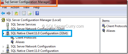
Step 1: Open the SQL Server Configuration Manager window through Start > All Programs > Microsoft SQL Server 2012 > Configuration Tools 



Step 2: Explore SQL Native Client 11.0 Configuration (32bit)



Step 3: Click on Client Protocols option within it  –



Step 4: Double click on TCP/IP from the right hand side pane



We will get to know the Default Port as shown here



The default port > 1433 port is the official Internet Assigned Number Authority (IANA) socket number for SQL Server. Client systems use TCP 1433 to connect to the database engine; SQL Server Management Studio (SSMS) uses the port to manage SQL Server instances across the network. You can reconfigure SQL Server to listen on a different port, but 1433 is by far the most common implementation.

Some other default SQL Server ports:

TCP 1434 – For Dedicated Admin Connection
UDP 1434 – For SQL Server Named Instance
TCP 2383 – For Default port of SSAS
TCP 2382 – For Named instances of SSAS
TCP 135 – For SSIS & T-SQL Debugger
TCP 80 and 443 – For SSRS
TCP 4022 – For Service Broker

SQL Server Alter Table with Add Column

There are many scenarios where we need to do structural changes to a table, i.e. adding a column, modifying data type, dropping a column and so on. This change to an existing table is possible by issuing a SQL Server Data Definition Language (DDL) T-SQL command known as Alter Table.

In this article we are specifically focusing on adding a new column in a table using SQL Server Alter Table.

Scenario 1: Adding columns to empty table

When the table is created and if there are no records in that table, then there is no problem in adding a column or multiple columns to that table.

Let us see the following example:

create table customers1
(
  custid varchar(5),
 custname varchar(50)
)
go

Scenario 1.a: Adding single column:

After creating the table, we realize that date of birth (DOB) column needs to be added. The following command will help us in achieving this.

Alter Table customers1
Add DOB Date
go

Scenario 1.b: Adding multiple columns:

Adding two more columns is also very easy. Let us add nationality and gender as two more columns by just having a comma separator in each definition.

Alter Table customers1
Add Nationality Varchar(40), Gender Char(1)
go

Scenario 1.c: Adding columns with constraints:

Adding a column with constraint such as primary key, unique key, foreign key, not null, check or default is again not challenging in an empty table.

Note – A primary key constraint cannot be added on the new column if there is already a primary key on any other existing column.

Let us add SSN and deposit amount as two columns, SSN having primary key and deposit amount having check constraint.

Alter Table customers1
Add SSN Varchar(10) Primary Key, 
Deposit_Amount Integer Check(Deposit_Amount >= 200)
go

Scenario 2: Adding columns to table having records

When a column is added to a table with existing records, then for those records, by default a null value is assigned by SQL Server.

Adding column on table having existing records.

Let us create table customers2 and add 2 records in it.

create table customers2
(custid varchar(5),
 custname varchar(50)
 )
 Go
Insert into customers2 Values('C1','John')
Insert into customers2 Values('C2','Martin')
go

Scenario 2.a: Adding columns with default null values on existing records.

Alter Table customers2
Add DOB Date
go

Let us see the table Customers2

select * from customers2

Image2-No-Default-Value

Scenario 2.b: Adding columns with default value

It might happen that you want to add a column specifying some default value and there are existing records in the table. But in the default setup, those existing records will not get that value.
Let us add token amount as a column to this Customers2 table with default value as 100.

Alter Table customers2
Add Token_Amount Integer Default 100
go

Let us see the table Customers2

select * from customers2

Image2-No-Default-Value

Note -The default value will be effective when new record is added.

Scenario 2.c: Adding columns with default value and applying those values on existing records.

Let us add another column tax with default value as 50. This value needs to be added to the existing records as well. We need to explicitly specify the clause With Values.

Alter Table customers2
Add Tax Integer Default 50 With Values
go

Image3-Default-Value-WithClause

Scenario 2.d: Adding columns with Not Null constraint on existing records.

Let us add a column Country with Not Null constraint. Now this will be contradictory because the earlier two records cannot have null value for Country.

Let us try.

Alter Table customers2
Add Country Varchar(50) Not Null
go

It will throw the following error.

ALTER TABLE only allows columns to be added that can contain nulls

To rectify this, we need to mention the default value which will safeguard the earlier records.

Scenario 2.e: Adding columns with not null constraint and default value on existing records

Let’s have India as the default value.

Alter Table customers2
Add Country Varchar(50) Default 'India' Not Null
go

Now this works fine. Let us see the table again.

select * from customers2

Image4-Default-Value-NotNull

Conclusion:

In this article, we have seen the following scenarios of using ALTER table to add column to a SQL Server table:

1. Adding one or multiple columns to an empty table.
2. Adding column to table having records. Those records get default value as null.
3. Adding column with default value to table having records

• In absence of With Values clause
• In presence of With Values clause

4. Adding column with not null constraint to table having records

• In absence of Default clause
• In presence of Default clause

T-SQL Date Format with Convert

In this article we are going to see a very handy SQL Server T-SQL function for formatting date called Convert(). It is generally used to show date values in different styles or formats.

Normally any date value when entered in a SQL Server table gets displayed in the default format as YYYY-MM-DD. Many a times, in your client application you may need to change the output of date & time for display purpose. For doing this the T-SQL Convert function is used.

Convert Function Example

Let us create a sample database Convert_Demo in our SQL Server database instance.

Use Master
go
Create Database Convert_Demo
go
Use Convert_Demo
go
CREATE TABLE EMP
       (EMPNO Integer Primary Key,
        ENAME Varchar(15),
        JOB Varchar(9),
        MGR Integer,
        HIREDATE date,
        SAL Integer,
        COMM Integer,
        DEPTNO Integer);
go
INSERT INTO EMP VALUES
        (7369, 'SMITH',  'CLERK',     7902, '12/17/80',
        800, NULL, 20);
INSERT INTO EMP VALUES
        (7499, 'ALLEN',  'SALESMAN',  7698,
        '5/20/81',1600,  300, 30);
INSERT INTO EMP VALUES
        (7521, 'WARD',   'SALESMAN',  7698,
        '5/22/81', 1250,  500, 30);
INSERT INTO EMP VALUES
        (7566, 'JONES',  'MANAGER',   7839,
        '4/2/81',  2975, NULL, 20);
INSERT INTO EMP VALUES
        (7654, 'MARTIN', 'SALESMAN',  7698,
        '9/28/81', 1250, 1400, 30);
INSERT INTO EMP VALUES
        (7698, 'BLAKE',  'MANAGER',   7839,
        '5/1/81',  2850, NULL, 30);
INSERT INTO EMP VALUES
        (7782, 'CLARK',  'MANAGER',   7839,
        '6/9/81',  2450, NULL, 10);
INSERT INTO EMP VALUES
        (7788, 'SCOTT',  'ANALYST',   7566,
        '12/9/82', 3000, NULL, 20);
INSERT INTO EMP VALUES
        (7839, 'KING',   'PRESIDENT', NULL,
        '11/17/81', 5000, NULL, 10);
INSERT INTO EMP VALUES
        (7844, 'TURNER', 'SALESMAN',  7698,
        '9/8/1981',  1500,    0, 30);
INSERT INTO EMP VALUES
        (7876, 'ADAMS',  'CLERK',     7788,
        '1/12/83', 1100, NULL, 20);
INSERT INTO EMP VALUES
        (7900, 'JAMES',  'CLERK',     7698,
        '12/3/81',   950, NULL, 30);
INSERT INTO EMP VALUES
        (7902, 'FORD',   'ANALYST',   7566,
        '12/3/81',  3000, NULL, 20);
INSERT INTO EMP VALUES
        (7934, 'MILLER', 'CLERK',     7782,
        '1/23/82', 1300, NULL, 10);
go

Now let us see the default presentation style of the hiredate column by executing the following SQL statement.

select ename, hiredate from emp

Image1-Default-date-format

Syntax of Convert function

CONVERT(data_type(length),data_to_be_converted,style)

Data_type(length) - varchar data type particulary for displaying dates in different format.

data_to_be_converted - The date value which needs to be converted.

Style - There are some predefined style ids like 101 for American date format, 103 in British format and so on. The style chart has been shown next –



Now let us see the employee names & hiredate in American as well as British formats using T-SQL Convert function.

select ename, hiredate as [Default Date Format],
convert(varchar, hiredate, 101) as [American],
convert(varchar, hiredate, 103) as [British] 
from emp

Image2-Changed-Date-Formats

Convert without StyleID:

Convert is also useful to convert from one data type to another – For example changing Float to Int, Number to Float or Number to Varchar.

Using Convert to change from Float to Int

SELECT CONVERT(int, 14.85)

Image3-Changing-Float-To-Int

Using Convert to change from Number to Float

SELECT CONVERT(float, 14.0989654)    

Image4-Number-to-Float

Using Convert to change from Number to Varchar

SELECT CONVERT(varchar(4), '12.3456')

Image5-Number-to-Varchar

Conclusion:

 

We have seen in this article that using T-SQL function Convert, we can display date in different formats and also can type cast one data type into another.

SQL Server CASE Statement and CASE WHEN Examples

Many a times there’s a need to create a derived column in an output, based on some condition. The condition is similar to the typical if construct we use if many programming languages.

In SQL scripting, we can use Case expressions or Case Statements as you may call them, to create a derived column based on a condition.

Also read about Nested Case Statements in SQL Server.

Let us first execute a sample database creation script that we will be using in our examples:

Use Master
go
Create Database Case_Demo
go
Use Case_Demo
go
CREATE TABLE EMP
       (EMPNO Integer,
        ENAME Varchar(15),
        JOB Varchar(9),
        MGR Integer,
        HIREDATE datetime,
        SAL Integer,
        COMM Integer,
        DEPTNO Integer)
go
INSERT INTO EMP VALUES
        (7369, 'SMITH', 'CLERK', 7902, '12/17/80', 800, NULL, 20)
INSERT INTO EMP VALUES
        (7499, 'ALLEN', 'SALESMAN', 7698, '5/20/81', 1600, 300, 30)
INSERT INTO EMP VALUES
        (7521, 'WARD', 'SALESMAN', 7698, '5/22/81', 1250, 500, 30)
INSERT INTO EMP VALUES
        (7566, 'JONES', 'MANAGER',   7839, '4/2/81', 2975, NULL, 20)
INSERT INTO EMP VALUES
        (7654, 'MARTIN', 'SALESMAN', 7698, '9/28/81', 1250, 1400, 30)
INSERT INTO EMP VALUES
        (7698, 'BLAKE', 'MANAGER',   7839, '5/1/81', 2850, NULL, 30)
INSERT INTO EMP VALUES
        (7782, 'CLARK', 'MANAGER',   7839, '6/9/81', 2450, NULL, 10)
INSERT INTO EMP VALUES
        (7788, 'SCOTT',  'ANALYST',  7566, '12/9/82', 3000, NULL, 20)
INSERT INTO EMP VALUES
        (7839, 'KING',   'PRESIDENT', NULL, '11/17/81', 5000, NULL, 10)
INSERT INTO EMP VALUES
        (7844, 'TURNER', 'SALESMAN', 7698, '9/8/1981',1500,    0, 30)
INSERT INTO EMP VALUES
        (7876, 'ADAMS', 'CLERK', 7788, '1/12/83', 1100, NULL, 20)
INSERT INTO EMP VALUES
        (7900, 'JAMES', 'CLERK', 7698,  '12/3/81', 950, NULL, 30)
INSERT INTO EMP VALUES
        (7902, 'FORD',   'ANALYST', 7566, '12/3/81', 3000, NULL, 20)
INSERT INTO EMP VALUES
        (7934, 'MILLER', 'CLERK',  7782, '1/23/82', 1300, NULL, 10)
go

There are two types of Case expressions:

1. Case acting as a Switch Case construct.
2. Case acting like an If…Else If….Else construct.

Switch Case Construct

Let us see an example of Case acting as a Switch Case construct.

The syntax is as follows:

Case Expression or Column Name
    When Value1 Then Statement1 or Expression 1
    When Value2 Then Statement2 or Expression 2
    When Value3 Then Statement3 or Expression 3
    .......................................................
    .......................................................
    When Value m Then Statement m or Expression m    
    Else
        Statement n or Expression n
End

Note: The Value above will be the actual value from a column, i.e. string or numeric or date value.

The Statement can be a string , numeric or date value. Expression can be either a derived value such as [Column Name] * 12 or using a T-SQL function Lower([Column Name])

Let us see an example to make things clearer.

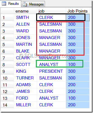
Let us display the employee name, job and job_points for each record. Now job_points will be a derived column based on a condition that says - If job is of Analyst then job_points will be 100, if it is clerk then 200, else for any other job type it will be 300.

select ename, job,  case job    
    when 'Analyst' then 100
    when 'Clerk' then 200
    else 300
         end as "Job Points"
from emp

Image 1: Case-As-Switch-Case


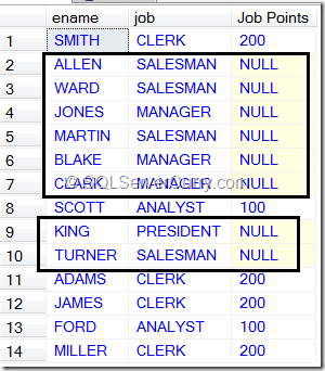
Else part is optional. If it is not mentioned, then NULL will be returned for the default values.
Let us see the same

select ename, job, case job    
    when 'Analyst' then 100
    when 'Clerk' then 200
    end as "Job Points"
from emp

Image 2: Case-Without Else

All the statements mentioned in the then clause should be of the same data type.

select ename, job, case job    
    when 'Analyst' then 100
    when 'Clerk' then 'Two Hundred'
    end as "Job Points"
from emp

The above query throws an error since at first the when clause is 100 i.e. a numeric value, but the next when clause has 'Two Hundred' as a value of string type.

The error message is as follows:

Msg 245, Level 16, State 1, Line 1 Conversion failed when converting the varchar value 'Two Hundred' to data type int.

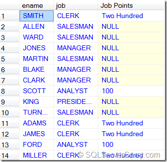
As I mentioned earlier, All the statements mentioned in the then clause should be of the same data type. So to fix this error, we need to enclose 100 in single quotes to make it a Varchar value.

select ename, job, case job    
    when 'Analyst' then '100'
    when 'Clerk' then 'Two Hundred'
    end as "Job Points"
from emp

Now we will get the desired output -


Image 3: Case-After-Rectification

IF ELSE Construct

Let us now see how to use the Case expression as an If…Else If….Else construct.
The syntax will be as follows:

Case 
    When Boolean Condition 1 Then Statement1 or Expression 1
    When Boolean Condition 2 Then Statement2 or Expression 2
    When Boolean Condition 3 Then Statement3 or Expression 3
    ........................................................
    ........................................................
    When Boolean Condition m Then Statement m    or Expression m
    Else
        Statement n or Expression n
End

Note: In this syntax, after the CASE keyword there is no Expression or Column Name. We directly have a When clause. The When clause will have a Boolean condition in which the column name or expression will be included.

Let us see an example of this.

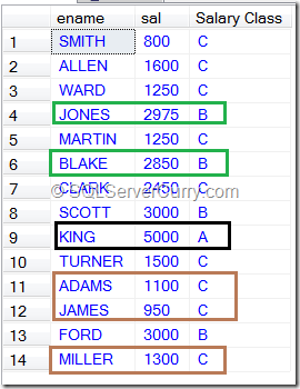
Let us create a query which will show employee name, salary and salary class. If the salary is greater than or equal to 5000 then salary class will be A, if it is between 2500 and 4999 then it will be B and for remaining salaries, values will be C.

select ename, sal, case 
    when sal >= 5000 then 'A'
    when sal >= 2500 then 'B'
    else
    'C'
           end as "Salary Class"
From Emp

Image 4: Case-If-Else

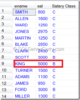
Note: The sequence of Boolean conditions will matter a lot. Whichever condition is true, its statement or expression gets executed and it comes out of the CASE expression for that record.

So if we swap the first two conditions in the above example, the output will go haywire.

Let us see an example

select ename, sal, case 
    when sal >= 3000 then 'B'
    when sal >= 5000 then 'A'
    else
    'C'
           end as "Salary Class"
From Emp

Image 5: Case-Logically-Wrong

Note: To avoid such logical errors, it will be better to avoid relational operators like >,>=. Instead use the between operator, mention the exact range and after doing this, if the conditions are given in any sequence, the output will be logically correct. Alternatively if you are going to continue with >,>= operators, then strictly all the conditions should be descending or all should be ascending.

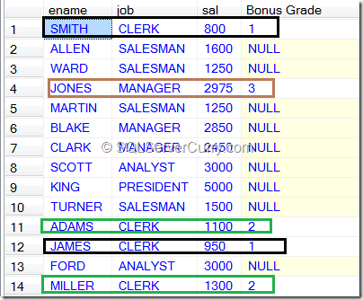
We can mention multiple conditions in each WHEN clause using logical and/or operators.

The following example will depict this point.

select ename, job, sal, case 
    when job = 'clerk' and sal < 1000 then '1'
    when job = 'clerk' and sal > 1000 then '2'
    when job = 'manager' and sal > 2900 then '3'
               end as "Bonus Grade"
From Emp

Image 6-Case-Multiple-Conditions-In-When

We explored the SQL Server CASE statement and also saw the CASE WHEN example. In the next article, we will explore Nested Case Statements in SQL Server. and use CASE in Having, Order By and UPDATE statements.

PIVOT and UNPIVOT in SQL Server

PIVOT and UNPIVOT are aggregate operators which are available from SQL Server version 2005 onwards.

PIVOT can be used to transform rows into columns while UNPIVOT can be used to transform columns into rows. We will see how to use PIVOT and UNPIVOT in the following examples

Let us create the following table which has sales details of products for each country.

create table #sales (country_name varchar(100),product_name varchar(100), 
sales_date datetime, sales_amount decimal(12,2))

insert into #sales (country_name,product_name,sales_date,sales_amount)
select 'India','Television','2012-01-10',35000 union all
select 'India','Mobile','2012-12-19',22000 union all
select 'India','Laptop','2012-04-11',62500 union all
select 'India','Laptop','2013-06-23',45000 union all
select 'India','Television','2012-03-20',45000 union all
select 'India','Television','2013-05-30',56000 union all
select 'India','Mobile','2013-02-22',71200 union all
select 'USA','Television','2012-02-20',3500 union all
select 'USA','Mobile','2012-11-01',2700 union all

select 'USA','Laptop','2012-08-19',6500 union all
select 'USA','Laptop','2013-06-23',5000 union all
select 'USA','Television','2012-02-12',4560 union all
select 'USA','Television','2013-06-30',5100 union all
select 'USA','Mobile','2013-006-06',2200 

SQL Server PIVOT table Example

Suppose you want to find out the total sales by each product and summarised for each year (ie columns are years). You can use the following code

SELECT product_name,[2012],[2013] from
(select year(sales_date) as sales_year,product_name,sales_amount FROM #sales)
as t 
PIVOT(SUM(sales_amount) 
      FOR sales_year IN ([2012],[2013])) AS pivot_table

If you want to group it by multiple columns, you can simply include that column in the query. For example the following query will do pivot group by country_name and product_name

SELECT country_name,product_name,[2012],[2013] from
(select year(sales_date) as sales_year, country_name, product_name, 
sales_amount FROM #sales) 
as t 
PIVOT(SUM(sales_amount) 
      FOR sales_year IN ([2012],[2013])) AS pivot_table

SQL Server UnPivot Table Example

To see how unpivot works, let us create the following table

create table #marks(student_name varchar(100), English smallint, 
Mathematics smallint, Tamil smallint, Science smallint)

insert into #marks(student_name , English, Mathematics, Tamil, Science)
select 'Sankar', 78,91,79,60 union all
select 'Nilesh', 81,90,66,89 union all
select 'Murugan', 94,88,72,90 

Suppose you want to transform the columns into rows i.e. subjects become rows, use the following query:

select student_name, subject_name, mark
from #marks s
unpivot
(
  mark
  for subject_name in (English,Mathematics, Tamil,Science)
) t;

Note : PIVOT in SQL Server basically produces a denormalised dataset whereas UNPIVOT produces normalised dataset.

CUBE and ROLLUP with GROUPBY in SQL Server

CUBE and ROLLUP are SQL Server operators which are always used along with a GROUP BY clause. These operators perform multi level aggregations at each column specified in the GROUP BY Clause. ROLLUP will do aggregation in the following manner:

Operation : ROLLUP(col1,col2)
Groupings : col1,col2
            col1, ALL(NULL)
            ALL (NULL)

CUBE will do aggregation in the following manner:

Operation : CUBE(col1,col2)
Groupings : col1,col2
            col1
        ALL(NULL), col2
            ALL(NULL)

Let us create the following dataset and explore the resultset:

create table #sales_data(region varchar(30), sales_date datetime, 

sales_amount decimal(12,2))

truncate table #sales_data
insert into #sales_data(region,sales_Date,sales_amount)
select 'South Asia', '2014-01-01',30000 union all
select 'South Asia', '2014-05-01',72000 union all
select 'South Asia', '2015-05-01',6700 union all
select 'North America', '2014-03-01',12500 union all
select 'North America', '2015-05-01',80000 union all
select 'North America', '2015-05-01',9000 union all
select 'Australia', '2014-02-01',88000 union all
select 'Australia', '2015-01-01',144000 union all
select 'Australia', '2015-05-01',178000 

Using ROLLUP

select region, year(sales_date) as sales_year, 

sum(sales_amount) as total_spent  from #sales_data
group by region, year(sales_date)
with ROLLUP

The result of the above statement is as follows:

region                         sales_year  total_spent
------------------------------ ----------- ---------------
Australia                      2014        88000.00
Australia                      2015        322000.00
Australia                      NULL        410000.00
North America                  2014        12500.00
North America                  2015        89000.00
North America                  NULL        101500.00
South Asia                     2014        102000.00
South Asia                     2015        6700.00
South Asia                     NULL        108700.00
NULL                           NULL        620200.00

As you can see, Grouping is done in three cases.

1. Grouping by the columns region and sales_year
2. Grouping by the columns region only
3. Grouping by no columns

Using CUBE

select region, year(sales_date) as sales_year, 

sum(sales_amount) as total_spent  from #sales_data
group by region, year(sales_date)
with CUBE

The result of the above statement is as follows:

region                         sales_year  total_spent
------------------------------ ----------- -----------------
Australia                      2014        88000.00
North America                  2014        12500.00
South Asia                     2014        102000.00
NULL                           2014        202500.00
Australia                      2015        322000.00
North America                  2015        89000.00
South Asia                     2015        6700.00
NULL                           2015        417700.00
NULL                           NULL        620200.00
Australia                      NULL        410000.00
North America                  NULL        101500.00
South Asia                     NULL        108700.00

As you can see, Grouping is done in four cases.

1. Grouping by the columns region and sales_year
2. Grouping by the column sales_year only
3. Grouping by the column region
4. Grouping by no columns

You can use both of these operators to achieve aggregation at multiple levels. CUBE performs more number of aggregations with multiple combination of the grouping columns.

If you just want to perform multiple groupings not excluding the first column, you can use ROLLUP, otherwise use CUBE.

Note: Usage of ROLLUP and CUBE in SQL Server are time-consuming options as they do groupings at multiple level. If you use a reporting tool to display the result, you should avoid doing it in SQL and do it in the reporting tool itself .

SQL Server 2012 - Binding Sequence to a Column‏

Continuing my series on SQL Server 2012, today we will learn about Sequence which is an object in SQL Server 2012 and can be used to generate customized sequence numbers. Although it is independent of objects, however an object can bind it. In this post, we will see how to use that as default value for a column

Create a sequence named my_seq

create sequence my_seq
    as int
    start with 1
    increment by 1
GO

Create a table in which one of the columns has a default value of my_seq

create table testing (col1 int, col2 int default next value for my_seq)

Now add some data to the table

insert into testing (col1)
select 34 union all
select 6

Select data from the table and see what col2 returns

select * from testing 



Col2 returns unique numbers. It should be noted that if the sequence is used by many objects, the value may not be sequential i.e. some values may be used somewhere else.

This way we can use sequence object to generate unique numbers like an identity column

OFFSET FETCH in SQL Server 2012

I have been exploring the new OFFSET-FETCH filter introduced in SQL Server 2012 and find it quite useful. In simple words, the OFFSET and FETCH clauses give you the capability to implement a paging solution by specifying the starting and ending set of rows to return.

Madhivanan has written a nice article on OFFSET-FETCH introducing this new feature over here: Pagination with OFFSET and FETCH NEXT in SQL Server 2012

In this article, I will list down some important points to consider while working with the OFFSET-FETCH clause in SQL Server 2012

• OFFSET indicates the number of rows to skip, FETCH indicates the rows to return after the skipped rows
• The TOP clause in SQL Server is similar to the FETCH clause except that it does not have skipping capability.
• However TOP supports PERCENT and WITH TIES, but OFFSET-FETCH does not.
• Any query that uses OFFSET-FETCH must also have an ORDER BY clause
• You can use OFFSET without FETCH, but not the opposite. With every FETCH clause, you need OFFSET clause
• The Filter has a singular and plural support. For example to fetch one row, you can use FETCH 1 ROW. Similarly to FETCH more than 1, you can specify the plural ROWS

Check out an OFFSET-FETCH example

Does my SQL Server Database Support Compression?

Some time back, Praveen Dabade had written a nice article on SQL Server Compressed Tables and Indexes in SQL Server where he explained how compression is now supported on ‘ROW and PAGE’ for tables and indexes. However did you know that compression is an enterprise-level feature?

How do determine what Enterprise Edition features are enabled on your database? Well you can use the sys.dm_persisted_sku_features DMV to find what Enterprise Edition features are
enabled on your database.

Learn more about Dynamic Management Views (DMV’s) here

Here’s the query for the same

SELECT feature_name,feature_id
FROM
sys.dm_db_persisted_sku_features;

Running this query will list all edition-specific features that are enabled in the current database. Some of the database changing features restricted to the SQL Server Enterprise or Developer editions are Compression, Partitioning, ChangeCapture etc.

This DMV is also useful in situations where you are planning to move a database from a higher to a lower edition. Eg: From Enterprise to Standard edition. Running the query will tell you if there are any Enterprise Edition features enabled that may not work when you move to a lower edition.

The DMV will return no rows if no features restricted to a particular edition are used by the database.

Error Handling in SQL Server with THROW

Continuing our series on SQL Server 2012, today we will talk about THROW. In versions prior to SQL Sever 2012, we used @@RAISE_ERROR to generate error messages dynamically or using the sys.messages catalog.

Consider the following example

SELECT ROUND(800.0, -3)

On executing this statement, you get the following error:



because the value does not fit into the decimal data type.

You can use @@RAISERROR to raise a message

BEGIN TRY
SELECT ROUND(800.0, -3)
END TRY
BEGIN CATCH
DECLARE @ErrorMsg nvarchar(1000), @Severity int
SELECT @ErrorMsg = ERROR_MESSAGE(),
@Severity = ERROR_SEVERITY()
RAISERROR (@ErrorMsg, @Severity, 1)
END CATCH

Note: The old syntax of RAISERROR syntax specifying the error number and message number got deprecated (RAISEERROR 50005 ‘Exception Occurred’). Instead the new syntax RAISEERROR(50005, 10, 1) allowed you to specify the messageid, severity and state). For new applications use THROW.

However in SQL Server 2012, there’s a better way to this without much efforts – THROW. Consider the following code

BEGIN TRY
SELECT ROUND(800.0, -3)
END TRY
BEGIN CATCH
THROW
END CATCH



As you can see, with just one word THROW, we were able to handle the error with grace and get a result too.

User Defined Functions in SQL Server

User Defined Functions play an important role in SQL Server. User Defined functions can be used to perform a complex logic, can accept parameters and return data. Many a times we have to write complex logic which cannot be written using a single query. In such scenarios, UDFs play an important role. For example, we can call user defined function in a where clause or use a user defined function in a JOIN [Where UDF returns a result set].

SQL Server supports two types of User Defined Functions as mentioned below –

- Scalar Functions – The function which returns a Scalar/Single value.
- Table Valued Functions – The function which returns a row set of SQL server Table datatype. Table Valued Functions can be written as –

• Inline Table
• Multi-statement Table

We will explore these functions today. I am using SQL Server 2012 for this demonstration, although you can use SQL Server 2005, 2008, 2008 R2 as well.

I have preconfigured Northwind database on my SQL Server instance. We will be using the following tables for creating different User Defined Functions –

• Customers
• Employees
• Orders
• Order Details
• Products

Let’s start querying the above table. Open a new Query window and write the following commands –

Scalar Function

We will now create a scalar function, which returns the number of orders placed by a given customer. Write the following code in your query pad –



The above function returns an integer value. To test this function, we will write some code as shown below –



Let us see another example which will fetch the number of orders processed by an employee for a given year. Write the following function in our query pad –



We will test this function with different years for an employee as shown below –

Table Valued Functions

Now let’s try an Inline Table valued function. Inline Table valued functions can return a row set using SQL Server Table datatype. You cannot perform addition logic in inline table valued functions. We will fetch the product details purchased by a customer as shown below –



To test this example we will use a select statement as shown below –



Another example of the Inline Table Valued Function is as shown below –



To test this function, we will use different years as shown below –




We will now see a Multi-Statement Table Valued Function. This function can be used to perform additional logic within the function. The code is as shown below –



To use the Multi-Statement Table Valued function, use this code –



There are couple of limitations you must consider before creating User Defined Functions. Some of them are as shown below –

• You cannot modify the state of the database using UDFs
• Unlike Stored Procedures, UDF can return only one single result set
• UDF does not support Try-Catch, @ERROR or RAISERROR function

Summary – User-defined functions are routines which perform calculations, receive one or more parameters and return either a scalar value or a result set. In this article, we saw how to create User Defined Functions. We also saw how to use Scalar functions and Table Valued Functions [Inline Table Valued Functions and Multi-Statement Table Valued Functions].

Download the source code of this article (Github)